TCOM 501 Homework 1
Solutions
Problem 3.1
A customer that carries out the order (eat in the restaurant) stays for 5 minutes (25
minutes). Therefore the average customer time in the system is
=T
5.05.05.0
+
=
25
15
minutes
Applying Little’s Theorem the average number in the system is
·=
N l
75
minutes
T
·=
5
=
15
Problem 3.3
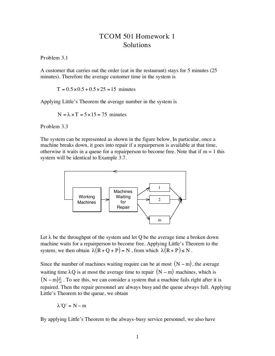
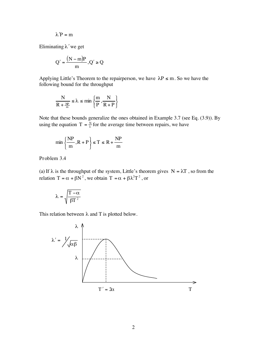
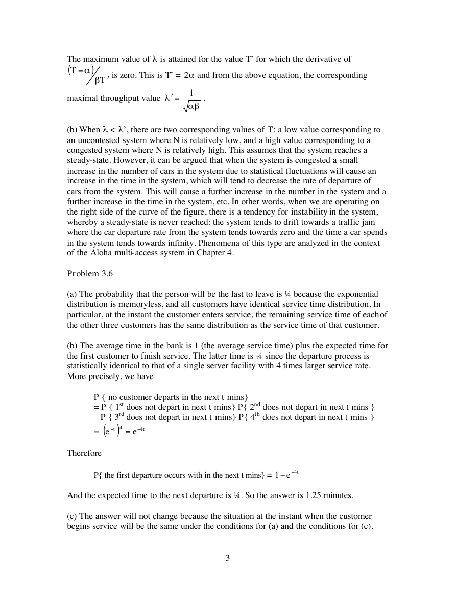
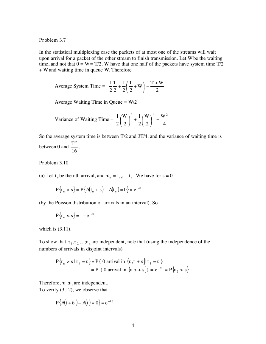
The system can be represented as shown in the figure below. In particular, once a
machine breaks down, it goes into repair if a repairperson is available at that time,
otherwise it waits in a queue for a repairperson to become free. Note that if m = 1 this
system will be identical to Example 3.7.
Working
Machines
Machines
Waiting
for
Repair
1
2
m
(
l
(
l
PQR
+
+
) N
=
, from which
Let l be the throughput of the system and let Q be the average time a broken down
machine waits for a repairperson to become free. Applying Little’s Theorem to the
+
PR
system, we then obtain
Since the number of machines waiting require can be at most (
waiting time lQ is at most the average time to repair (
)mN -
)
(
PmN -
repaired. Then the repair personnel are always busy and the queue always full. Applying
Little’s Theorem to the queue, we obtain
By applying Little’s Theorem to the always-busy service personnel, we also have
) N
.
)mN -
, the average
machines, which is
. To see this, we can consider a system that a machine fails right after it is
=¢
mNQ
¢l
m
1
·
·
£
-
�
mP =¢l
Eliminating l¢ we get
)
PmN
=¢
Q
(
m
,
QQ
Applying Little’s Theorem to the repairperson, we have
following bound for the throughput
mP £l
. So we have the
N
+
R
NP
m
l
min
m
P
,
N
+
PR
Note that these bounds generalize the ones obtained in Example 3.7 (see Eq. (3.9)). By
using the equation
T = for the average time between repairs, we have
N
l
min
NP
m
+,
PR
T
+
R
NP
m
Problem 3.4
(a) If l is the throughput of the system, Little’s theorem gives
relation
, we obtain
ba +
a +=
, or
2N
bl
=
2
2T
T
T
N l=
T
, so from the
=
l
a
T
2T
b
This relation between l and T is plotted below.
1=¢
l
l
ab
l
a2=¢T
T
2
‡
¢
-
£
£
£
£
-
�
The maximum value of l is attained for the value T’ for which the derivative of
(
T
is zero. This is T’ = 2a and from the above equation, the corresponding
a-
)
b
2T
maximal throughput value
l
1=¢
ab
.
(b) When l < l’, there are two corresponding values of T: a low value corresponding to
an uncontested system where N is relatively low, and a high value corresponding to a
congested system where N is relatively high. This assumes that the system reaches a
steady-state. However, it can be argued that when the system is congested a small
increase in the number of cars in the system due to statistical fluctuations will cause an
increase in the time in the system, which will tend to decrease the rate of departure of
cars from the system. This will cause a further increase in the number in the system and a
further increase in the time in the system, etc. In other words, when we are operating on
the right side of the curve of the figure, there is a tendency for instability in the system,
whereby a steady-state is never reached: the system tends to drift towards a traffic jam
where the car departure rate from the system tends towards zero and the time a car spends
in the system tends towards infinity. Phenomena of this type are analyzed in the context
of the Aloha multi-access system in Chapter 4.
Problem 3.6
(a) The probability that the person will be the last to leave is ¼ because the exponential
distribution is memoryless, and all customers have identical service time distribution. In
particular, at the instant the customer enters service, the remaining service time of each of
the other three customers has the same distribution as the service time of that customer.
(b) The average time in the bank is 1 (the average service time) plus the expected time for
the first customer to finish service. The latter time is ¼ since the departure process is
statistically identical to that of a single server facility with 4 times larger service rate.
More precisely, we have
P { no customer departs in the next t mins}
= P { 1st does not depart in next t mins} P{ 2nd does not depart in next t mins }
P { 3rd does not depart in next t mins} P{ 4th does not depart in next t mins }
= (
e
=
)
e
4
t
4
t
Therefore
P{ the first departure occurs with in the next t mins} =
1
te 4
And the expected time to the next departure is ¼. So the answer is 1.25 minutes.
(c) The answer will not change because the situation at the instant when the customer
begins service will be the same under the conditions for (a) and the conditions for (c).
3
-
-
-
-
�
Problem 3.7
In the statistical multiplexing case the packets of at most one of the streams will wait
upon arrival for a packet of the other stream to finish transmission. Let W be the waiting
time, and not that 0 = W = T/2. W have that one half of the packets have system time T/2
+ W and waiting time in queue W. Therefore
Average System Time =
1
T
22
+
1
T
22
+
W
=
Average Waiting Time in Queue = W/2
WT
+
2
Variance of Waiting Time =
1
W
22
2
+
1
W
22
2
=
2
W
4
So the average system time is between T/2 and 3T/4, and the variance of waiting time is
between 0 and
2T
16
.
Problem 3.10
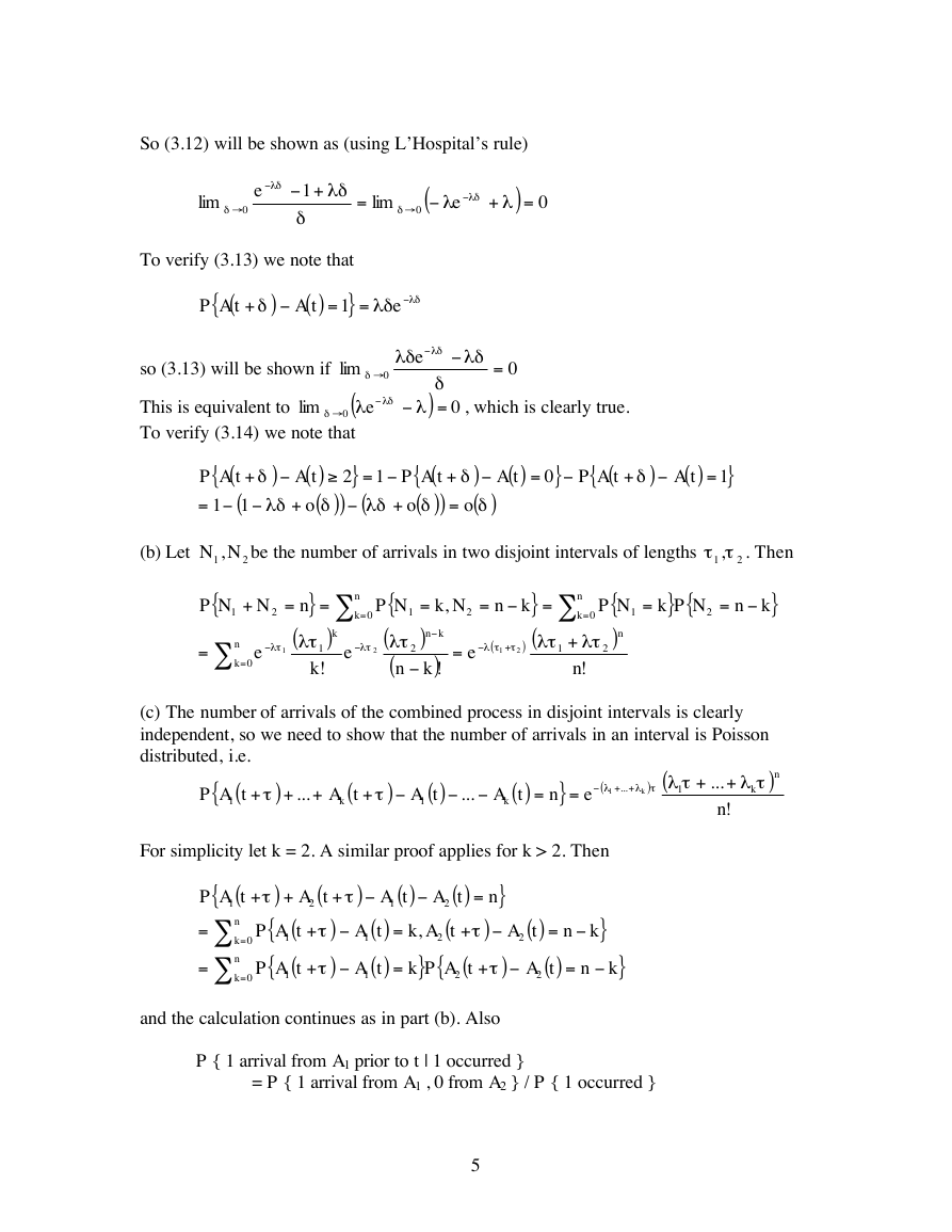
(a) Let nt be the nth arrival, and
)
(
{
tAP
P
}
s
{
t
+
=
>
s
n
. We have for s = 0
n
t
n
n
= +1
t
(
)
tA
=
n
0
t
}
-=
e
l
s
n
n
e
P
l
s
{
t
,...,
}
s
-=
1
tt
,
1
(by the Poisson distribution of arrivals in an interval). So
which is (3.11).
To show that
numbers of arrivals in disjoint intervals)
Therefore,
are independent.
To verify (3.12), we observe that
]
P{ 0 arrival in (
}=
tt
,
|
s
t
]s+tt ,
= P { 0 arrival in (
{
t
P n
(
{
tAP
( )
tA
|s
1,tt
-=
e
}
0
nt
+
t
1
+
d
ld
=
>
=
)
2
2
4
are independent, note that (using the independence of the
1
=
t
t
}
l
e s
} =
=
{
2t
P
>
}s
ł
Ł
ł
Ł
ł
Ł
-
-
-
£
-
-
�
So (3.12) will be shown as (using L’Hospital’s rule)
) 0
=
lim
lim
ld
l
e
+
=
+
(
l
e
ld
ld
d
0
d
0
1
d
To verify (3.13) we note that
}
1
(
{
tAP
( )
tA
=
+
d
)
=
ld
e
ld
e
ld ld
d
) 0
=
l
ld
=
0
, which is clearly true.
(
{
tAP
( )
)
+
d
o
+
=
d
o
( )
tA
)
( )d
=
}
0
(
{
tAP
)
+
d
( )
tA
=
}
1
d
so (3.13) will be shown if
lim 0
(
l ld
This is equivalent to
lim 0
e
To verify (3.14) we note that
}
( )
tA
2
( )
)
+
d
o
{
(
+
tAP
(
-=
1
1
)
d
ld
-=
1
(
ld
d
(b) Let
1,NN
{
NP
1
+
N
2
=
lt
n
k
=
0
e
1
be the number of arrivals in two disjoint intervals of lengths
2
1,tt
2
. Then
=
)
}
n
=
(
lt
1
k
!
k
n
k
=
0
lt
e
{
NP
(
lt
(
n
2
1
2
=
)
k
,
Nk
kn
=
)
!
-=
=
}
kn
) (
lt
+
t
2
(
tl
1
2
e
=
} {
NPk
2
1
-=
kn
}
{
NP
)
n
2
n
=
0
k
+
lt
n
!
1
(c) The number of arrivals of the combined process in disjoint intervals is clearly
independent, so we need to show that the number of arrivals in an interval is Poisson
distributed, i.e.
)
{
(
+
tAP
++
) (
tl
k
tl
1
++
...
...
...
tl
k
}
(
l
1
=
=
+
n
)
)
e
t
t
( )
tA
k
( )
tA
1
(
tA
k
1
n
++
...
!
n
For simplicity let k = 2. A similar proof applies for k > 2. Then
1
{
(
tAP
=
n
k
n
k
=
=
=
0
0
+
)
+
t
{
(
tAP
(
{
tAP
1
1
(
tA
2
+
t
+
t
+
)
)
t
}
( )
)
( )
tA
tA
1
2
( )
(
=
+
tAk
tA
,
1
}
( )
(
{
tAPk
tA
1
=
2
2
=
n
)
t
+
t
2
( )
tA
)
-=
( )
tA
2
kn
-=
n
}
}
k
and the calculation continues as in part (b). Also
P { 1 arrival from A1 prior to t | 1 occurred }
= P { 1 arrival from A1 , 0 from A2 } / P { 1 occurred }
5
-
-
-
fi
-
fi
-
-
-
-
fi
-
-
fi
-
-
-
-
-
‡
-
-
-
-
-
-
-
-
-
-
-
-
-
-
-
-
�
l
1
=
l
t
1
te
l
te
e
l
t
l
2
t
=
l
1
l
2
(d) Let t be the time of arrival. We have
P { t < s | 1 arrival occurred }
= P { t < s , 1 arrival occurred } / P { 1 arrival occurred }
= P { 1 arrival occurred in [t1, s), 0 arrivals occurred in [s, t2] }
(
l
=
s
l
)
l
/ P { 1 arrival occurred }
)
et
t
1
1
(
t
t
1
(
ts
1
)
et
1
ts
)
s
t
e
(
t
=
t
1
l
l
2
2
(
)
2
2
This shows that the arrival time is uniformly distributed in [t2, t2].
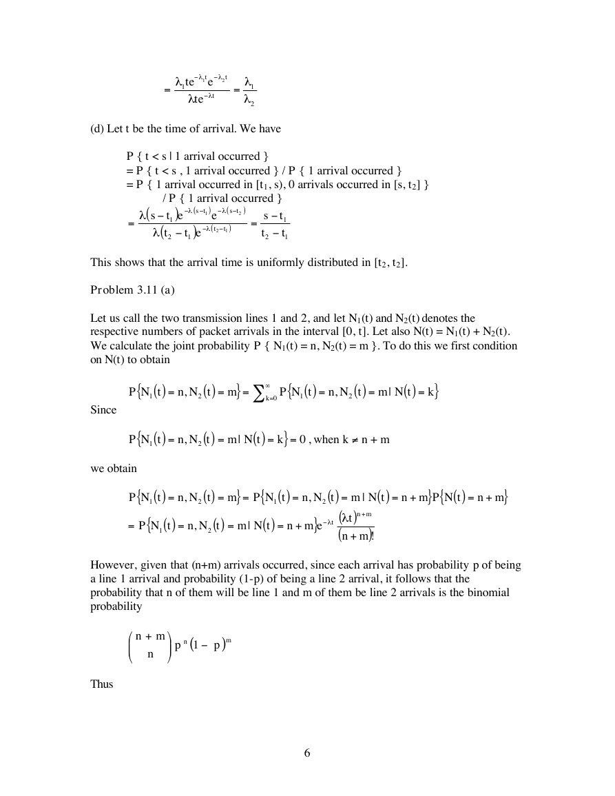
Problem 3.11 (a)
Let us call the two transmission lines 1 and 2, and let N1(t) and N2(t) denotes the
respective numbers of packet arrivals in the interval [0, t]. Let also N(t) = N1(t) + N2(t).
We calculate the joint probability P { N1(t) = n, N2(t) = m }. To do this we first condition
on N(t) to obtain
{
( )
tNP
Since
we obtain
( )
{
=
tNP
{
( )
tNP
{
( )
,
tNPmtNn
( )
tNm
( )
,
tNmtNn
( )
,
tNmtNn
( )
=
( )
,
tNn
}
,
mtNn
( )
( )
tNPmn
( )
tNm
( )
{
tNP
+=
}
mn
+=
}
emn
( )
,
tNn
{
( )
tNP
, when k „
} 0
=
n + m
+=
( )
}
}
{
}
=
=
=
=
0
k
=
=
=
k
2
2
=
1
1
1
=
=
|
=
=
=
=
1
2
k
|
2
2
=
1
1
|
2
|
+
mn
( )
=
(
)
ll
t
t
(
+
mn
)!
However, given that (n+m) arrivals occurred, since each arrival has probability p of being
a line 1 arrival and probability (1-p) of being a line 2 arrival, it follows that the
probability that n of them will be line 1 and m of them be line 2 arrivals is the binomial
probability
Thus
mn
+
n
(
1
n
p
)m
p
6
-
-
-
-
-
-
-
-
-
-
-
-
-
¥
-
-
ł
Ł
�
Hence
=
{
( )
tNP
1
(
l
tp
!
n
=
l
tp
e
2
=
( )
}
mtNn
,
(
)
l
t
n
)
(
1
l
p
t
e
mn
+
n
)
)
p
m
=
(
1
!
m
(
1
n
p
)
m
ep
l
t
+
mn
(
)
l
t
(
+
mn
)
!
=
( )
{
tNP
(
l
l
tp
1
=
e
}
n
)
tp
!
n
n
=
=
0
m
e
=
m
0
{
( )
tNP
(
l
(
1
l
1
p
)
t
( )
,
tNn
)
)
m
=
2
(
1
p
!
m
t
=
}
m
=
e
l
tp
(
l
n
)
tp
!
n
That is, {N1(t) = n, t > 0 }is a Poisson process having rate lp. Similarly we argue that
{N2(t) = m, t > 0 } is a Poisson process having rate l(1-p). Finally from Eq. (1) it follows
that the two processes are independent since the joint distribution factors into the
marginal distributions.
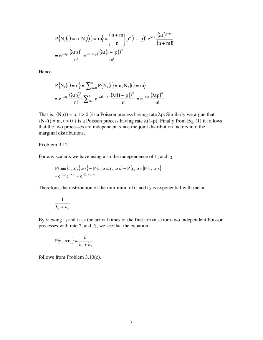
Problem 3.12
For any scalar s we have using also the independence of t 1 and t 2
} {
t
Ps
}
s
}
s
{
t
{
t
}
P
s
,
=
t
2
1
2
1
{
P
min
=
l
s
e
1
{
tt
,
1
l
s
e
2
}
2
=
e
=
s
(
+
ll
1
2
P
)s
Therefore, the distribution of the minimum of t 1 and t 2 is exponential with mean
1
l +
1
l
2
By viewing t 1 and t 2 as the arrival times of the first arrivals from two independent Poisson
processes with rate ?1 and ?2, we see that the equation
}
=
{
t
P
1
t
2
l
1
+
l
1
l
2
follows from Problem 3.10(c).
7
-
-
ł
Ł
-
-
-
-
-
¥
-
-
-
¥
-
-
-
-
‡
‡
‡
‡
‡
£
�
TCOM 501 Homework 2
Solutions
(
-1n
Problem 3.11(b)
Let A, A1, and A2 as in the hint. Let I be the interarrival interval of A2 and consider the
number of arrivals of A1 that lie in I. The probability that this number is n is the
)r
r
probability of n successive arrivals of A1 followed by an arrival of A2, which is
This is also the probability that a customer finds upon arrival n other customers waiting
in an M/M/1 queue. The service time of each of these customers is exponentially
distributed with parameter m , just like the interarrival times of process A. Therefore the
waiting time of the customer in the M/M/1 system has the same distribution as the
interarrival time of process A2. Since by part (a), the process A2 is Poisson with
rate
exponentially distributed with parameter
Problem 3.14
(a) The average message transmission time is
, it follows that the waiting time of the customer in the M/M/1 system is
C=m
lm -
lm -
. When
the number of packets in the system is larger than K, the arrival rate is 1l . We must
have
, so the service rate is
1
m
L
L=
C
.
.
0
0
l
1
l
2
m
in order for the arrival rate at node A to be less than the service rate for large state
values. For these values, therefore, the average number of packets in the system will
stay bounded.
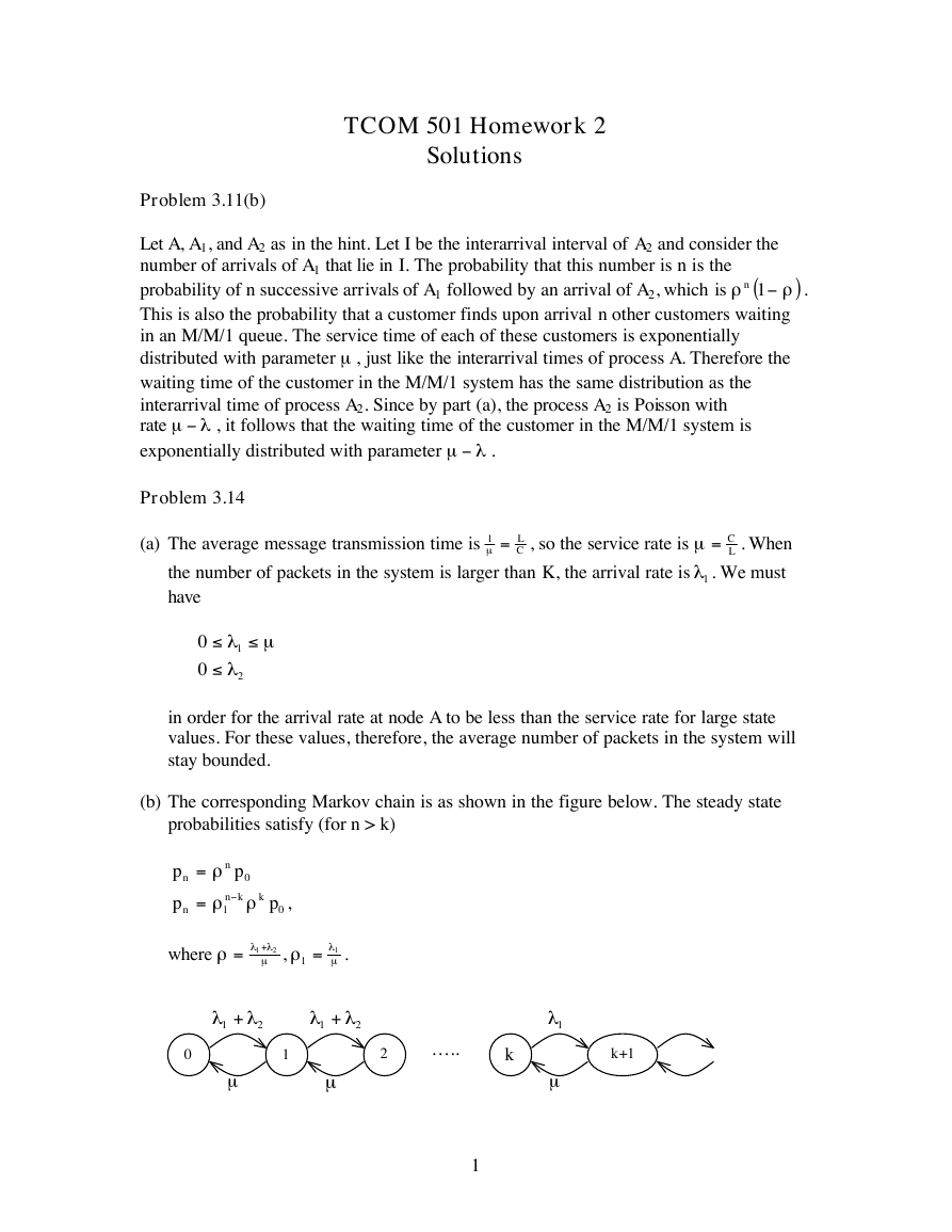
(b) The corresponding Markov chain is as shown in the figure below. The steady state
probabilities satisfy (for n > k)
r
r
n
p
kn
1
0
r
k
,0
p
=
=
p
p
n
n
where
r
= +
ll
2
1
m
,
r
1
=
l
1
m
.
0
l +
1 l
2
l +
1 l
2
1
m
m
2
…..
k
1l
m
k+1
1
£
£
£
-
�


 2023年江西萍乡中考道德与法治真题及答案.doc
 2012年重庆南川中考生物真题及答案.doc
 2013年江西师范大学地理学综合及文艺理论基础考研真题.doc
 2020年四川甘孜小升初语文真题及答案I卷.doc
 2020年注册岩土工程师专业基础考试真题及答案.doc
 2023-2024学年福建省厦门市九年级上学期数学月考试题及答案.doc
 2021-2022学年辽宁省沈阳市大东区九年级上学期语文期末试题及答案.doc
 2022-2023学年北京东城区初三第一学期物理期末试卷及答案.doc
 2018上半年江西教师资格初中地理学科知识与教学能力真题及答案.doc
 2012年河北国家公务员申论考试真题及答案-省级.doc
 2020-2021学年江苏省扬州市江都区邵樊片九年级上学期数学第一次质量检测试题及答案.doc
 2022下半年黑龙江教师资格证中学综合素质真题及答案.doc