v. 11.2
SMS 11.2 Tutorial
ADCIRC Analysis
Objectives
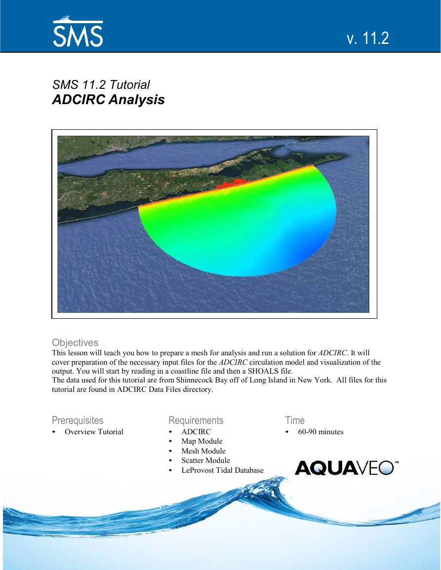
This lesson will teach you how to prepare a mesh for analysis and run a solution for ADCIRC. It will
cover preparation of the necessary input files for the ADCIRC circulation model and visualization of the
output. You will start by reading in a coastline file and then a SHOALS file.
The data used for this tutorial are from Shinnecock Bay off of Long Island in New York. All files for this
tutorial are found in ADCIRC Data Files directory.
Prerequisites
• Overview Tutorial
Requirements
• ADCIRC
• Map Module
• Mesh Module
• Scatter Module
• LeProvost Tidal Database
Time
• 60-90 minutes
�
coastline arc to select it.
3. Select Feature Objects | Define Domain.
4. Select the Semi-circular option and click OK.
5. Frame
the display.
A semi-circular arc is created to define the region.
1.2 Assigning Boundary Types
1 Reading in a Coastline File
For this tutorial, you will first read in a coastline file, which has already been set up for
you. This sample coastline will form the boundary for your mesh. To set up your
coverage for ADCIRC and open the coastline file:
1. Change the coverage type to ADCIRC by right clicking on default
coverage, selecting Type, and choosing ADCIRC (in the models subcategory).
Select File | Open.
Select the file shin.cst in the Data Files Folder for this tutorial and click the
Open button.
2.
3.
Coastline files include lists of two-dimensional polylines that may be closed or open. The
open polylines are converted to Feature Arcs and are interpreted as open sections of
coastline. Closed polylines are converted to arcs and are assigned the attributes of islands.
1.1 Defining the domain
We need to assign a boundary type to the coastline arc, and then we can define the region
to be modeled. To do this:
1. Make sure you are in the Map
module, if not already selected.
2. Choose the Select Feature Arc
tool from the Toolbar and click on the
Boundary types for arcs are specified in the Map module. Boundary types are prescribed
by setting attributes to Feature Arcs. To set the boundary types:
1. Choose the Select Feature Arc
tool from the Toolbox.
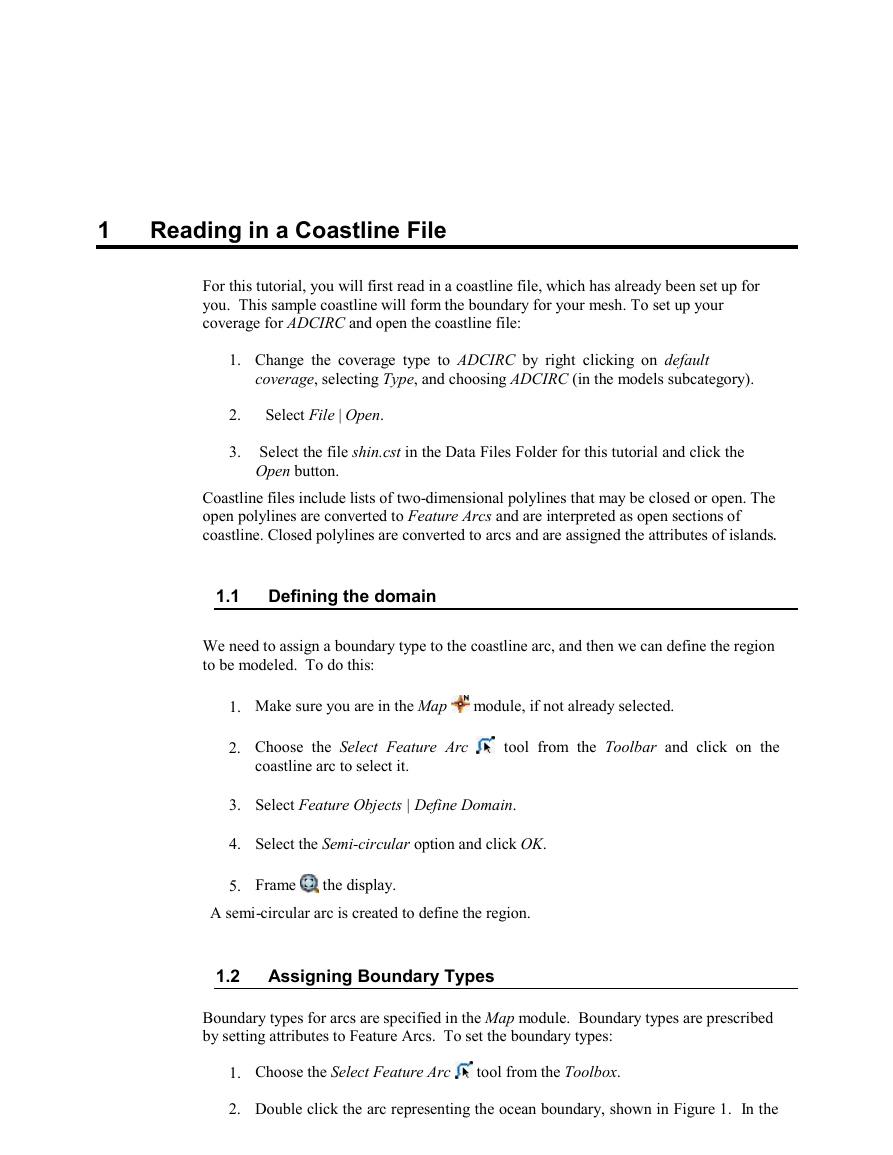
2. Double click the arc representing the ocean boundary, shown in Figure 1. In the
�
ADCIRC Arc / Nodestring Attributes dialog, assign this arc to be of type Ocean.
3. Click the OK button to close the dialog.
2
Feature Arcs after boundary types have been assigned
Figure 1
*Note: When the Coastline file is read into a coverage that is already set as a ADCIRC
type, it will automatically be read in as a Mainland boundary arc. If you set the coverage to
type ADCIRC after you have read in the coastline file, you will have to double click on the
coastline arc and set it to be a mainland boundary.
Editing the Coastline File
Now that the coastline file has been read in and a corresponding map object created,
several modifications must be made to the data before the SHOALS file is read in. Since
the SHOALS file is in UTM coordinates, zone 18(78W to 72 W northern Hemisphere), the
data should also be set to those coordinates. In order to do this the display projection must
be set to same global projection. To convert the display coordinates:
1. Choose Display | Projection….
2. In the Display Projection dialog that appears, toggle on Global projection and
click Set Projection. Set the projection to UTM, and set the zone to 18 ( 78W to
72W – Northern Hemisphere) and the datum as NAD 27. Click OK.
3. Ensure that the vertical units is set to Meters.
4. Click the OK button to exit the dialog. Next, to set the Map object coordinates:
5. Right-click on the "default coverage" map object and select Projection.
6. Click "Set Projection: and set projection to Geographic (Latitude/Longitude)".
�
7.
Right-click Default Coverage again and select Work in Object Projection.
8. Right-click the Default Coverage again and select Reproject. The current
projection should be set to Geographic and the new projection should
be set to UTM with zone 18 and the Datum set at NAD27. Click OK. (Click the
Frame macro to see the points.)
The coastline data has now been converted to a global projection of UTM coordinates with
zone 18 (78w to 72W--Northern Hemisphere) and Datum set at NAD27. However, the
display projection is now in Geographic (Latitude/Longitude). Before reading in the
SHOALS data we must first change it back to UTM. To do this:
1. Right-click on the default coverage and select Work in Object Projection.
3 Reading in a SHOALS File
You will now read in a SHOALS file, shin.pts, which contains data at various locations
along the coastline and throughout the region you are modeling.
1. Choose File | Open.
2. Select the file shin.pts.
3. In the Open File Format dialog, toggle on Use Import Wizard and click OK.
The File Import Wizard dialog will open, allowing you to specify how the data will be
read into SMS. For Step 1 of the dialog, the first line in the File preview box is the file
header. The next line shows the name of each respective column of data. In this case,
the file has three data columns. The first column is the X Coordinate, the second column
is the Y Coordinate, and the third column is the depth/bathymetry.
• Click the Next > button to move on to Step 2 of the File Import Wizard.
The second step of the File Import Wizard allows you to change other specifications as
you read in the SHOALS file.
• Click the Finish button.
Figure 2 shows the plot of the points read in from the shin.pts file. (If the scatter set does
not appear at first, make sure that Points is toggled on in the display options under
Scatter).
Once the scatter set is read in, we must set its projection. To do this:
1. Right click on the shin scatter set in the project explorer, and click on projection.
2. In the Object Projection dialog, the projection will already be set to UTM since
the Display Projection is currently set to UTM. Click OK to exit the dialog.
�
4
Figure 2
Display of shin.pts.
Shallow Wavelength Functions
The next step before you build your finite-element mesh is to create several functions for
creating the finite element mesh. For this tutorial, the mesh will be generated according to
the wavelength at each node. Large elements will be created in regions of long
wavelengths. Conversely, smaller elements are needed closer to the shore to correctly
model the smaller wavelengths.
To create this shallow wavelength function from the bathymetric data:
1. In the Scatter
module, select Data | Data Set Toolbox.
2. In the Data Set Toolbox dialog, select the Wavelength and Celerity tool in the
Coastal section. This enables the wavelength options on the dialog.
3. Make sure the options for creating a Wavelength and Celerity function are
checked. Leave the period at 20 seconds and enter a name “20 sec” in the Output
data set names edit field.
4. Click the Compute button to create the data sets and the Done button to close the
dialog.
Two functions are created: celerity and wavelength at each node using the shallow water
wavelength equation. The celerity is calculated as:
Celerity = (Gravity * Nodal Elevation)0.5.
•
The wavelength is calculated as:
• Wavelength = Period * Celerity.
�
5 Creating Size Functions
Now that you have created the wavelength function, you must make a few more
conversions before you are ready to create your mesh. A size function is a multiple that
guides the size of elements to be created in SMS. Any data set may be used for this
purpose. If you were to generate your mesh using the original wavelength function alone,
you would get a decent mesh to work with, but we want a mesh whose density radiates
out from a point in the inlet. This allows you to get more accurate results in the inlet
where we are most concerned with the outcome of the ADCIRC run. Therefore, we will
now need to create a size function based on the wavelength to attain this end. The final
size function you use for modeling applications varies and is found through trial and error
to give a nicely formed mesh. This example illustrates one method of building a size
function.
5.1
Finding the Central Point for the Mesh
Since the mesh will be generated in a radial fashion, the distance from a central point
must be found. The first step is to locate the central point and then use the Data
Calculator to compute the distances of all points from this center point. To do this:
1. Still in the Scatterpoint
Figure 3 with the Zoom
module, zoom in to the area of the inlet shown in
tool until your screen looks like Figure 4.
2. Click on one of scatter points in the middle of the inlet using the Select
tool. Make note of this point’s X and Y coordinates in the Edit
Scatterpoints
Window at the top of the screen.
3. Frame the data by clicking the Frame
tool in the Toolbox.
�
Figure 3
Inlet location to zoom in on.
Figure 4 Choose a center point.
For now, turn off the scatterpoint display. However, you may turn it back on at any
time during the tutorial if you so desire. To turn off the visibility of the shin.pts data
unselect the box next to the
You are now ready to proceed. We will use the Data Calculator to compute new
data sets by performing operations with scalar values and existing data sets. The
Data Calculator will be used to create the size function.
shin dataset in the Project Explorer.
�
5.2 Distance Function
For consistency, we will use the (x,y) location of (712768.675, 4523969.712) as
the center scatterpoint for our mesh.
1. Select Data | Data Calculator…. This brings up the Dataset Toolbox, with
the data calculator active.
2. Click the sqrt(x) button.
3. In the Expression field, using the keyboard replace “??”so the expression
looks like:
sqrt((d4 – 712768)^2 + (d5 – 4523950)^2)
•
This expression takes the x and y locations of each scatter point, which correspond to
the “d4” and “d5” data sets respectively, and computes its distance to the point
designated as the mesh center.
4. In the Output data set name field, enter the name of “distance” for the data
set and click the Compute button.
5.3
Initial Size Function
1. Highlight the “20 sec_Wavelength” data set and click the Add to
Expression button. You now should see the letter and number “d2” in the
Expression field.
2. In the Expression field, make the equation look like “d2*7”.
3. Enter the name “size” for this data set in the Output dataset name area and
click the Compute button. This creates a function of 7 times the wavelength.
5.4 Scale Function
scale = (distance/max distance)^0.5.
The last separate function before computing the final size function will be a scale
factor out from the center point. It will take on the following format:
•
This scale function will range between 0 and 1, 0 being at the center point and 1 at the
farthest point from the center of the mesh. This will allow the mesh to radiate out in
density from the middle of the inlet. Taking the square root of the scale factor forces
the elements to grow larger more quickly as one moves away from the center. To
compute this function:
1. Highlight the “distance” function in the Data Sets window and click the Data
Set Info... button. Notice that the Maximum value is 65607.9.
2. Click the X in the corner of the dialog window to close the info dialog.
�



 2023年江西萍乡中考道德与法治真题及答案.doc
 2012年重庆南川中考生物真题及答案.doc
 2013年江西师范大学地理学综合及文艺理论基础考研真题.doc
 2020年四川甘孜小升初语文真题及答案I卷.doc
 2020年注册岩土工程师专业基础考试真题及答案.doc
 2023-2024学年福建省厦门市九年级上学期数学月考试题及答案.doc
 2021-2022学年辽宁省沈阳市大东区九年级上学期语文期末试题及答案.doc
 2022-2023学年北京东城区初三第一学期物理期末试卷及答案.doc
 2018上半年江西教师资格初中地理学科知识与教学能力真题及答案.doc
 2012年河北国家公务员申论考试真题及答案-省级.doc
 2020-2021学年江苏省扬州市江都区邵樊片九年级上学期数学第一次质量检测试题及答案.doc
 2022下半年黑龙江教师资格证中学综合素质真题及答案.doc