submittedforpublication
1
Feature Extraction from Point Clouds
Stefan Gumhold�
Xinlong Wangy
Rob MacLeodz
Scientific Computing and Imaging Institute
University of Salt Lake City, Utah
Figure 1: a) input point cloud. b) the neighbor graph. c) point classification. d) crease pattern forming. e) purified crease pattern. f) spline
representation of crease pattern
Abstract
This paper describes a new method to extract feature lines directly
from a surface point cloud. No surface reconstruction is needed
in advance, only the inexpensive computation of a neighbor graph
connecting nearby points.
The feature extraction is performed in two stages. The first stage
constists of assigning a penalty weight to each point that indicates
the unlikelihood that the point is part of a feature and assigning
these penalty weights to the edges of a neighbor graph. Extracting
a subgraph of the neighbor graph that minimizes the edge penalty
weights then produces a set of feature patterns. The second stage
is especially useful for noisy data.
It recovers feature lines and
junctions by fitting wedges to the crease lines and corners to the
junctions.
As the method works on the local neighbor graph only, it is fast
and automatically adapts to the sampling resolution. This makes
the approach ideal as a preprocessing step in mesh generation.
CR Categories:
detection]—;
Keywords: feature detection, scattered data
I.4.6 Segmentation [Edge and feature
1 Introduction
In this paper we consider the feature detection and reconstruction
problem for the case of the input surface being described by a point
cloud. Figure 2 illustrates for the surface of the well known Stan-
ford bunny the different types of feature elements that we want to
extract. The crease pattern, shown in dark blue, consists of crease
lines that either terminate in junctions or singleton ends or they
close to form a loop. The border pattern consists only of border
loops.
Input points that lay on a crease are called crease points,
points on the border loops are border points. At a junction the cor-
responding data point is called a corner or junction point and at
singleton ends we find end points. The feature extraction algorithm
�stefan@gumhold.com
ywangxl@cs.utah.edu
zmacleod@cvrti.utah.edu
Figure 2: different elements in the crease and border patterns
that we describe here is fully automated and no seed or junction
points need to be marked by the user.
Figure 1 illustrates our feature extraction pipeline. The input
is a point cloud a); in this case the underlying surface is a model
of the human torso. In the analysis stage we construct a neighbor
graph b) on the point cloud that reflects proximity. The classifica-
tion stage that follows fits ellipsoids c) to the neighborhoods of the
input points, approximates the surface curvature and the maximum
open angle; the latter is used to detect border points. From these
vertex properties we define crease and border penalty weights that
measure the unlikelihood that a specific point is on a crease or bor-
der line, respectively. From the penalty weights at the vertices we
compute penalty weights at the edges of the neighbor graph. The
feature line linkage stage finds spanning patterns in the neighbor
graph that minimize the crease or border penalty weights, respec-
tively. A minimum crease spanning pattern is shown in d). The
minimum spanning pattern is similar to a minimum spanning tree
but allows for significantly long cycles. A pruning algorithm cuts
off short branches e). For noisy data the resulting crease lines are
jittered because no input points lay directly on the actual crease
line, in which case we apply a crease line and junction recovery al-
gorithm. This algorithm fits wedges, a simple crease representation
consisting of two half planes meeting at a line, to the crease neigh-
�
submittedforpublication
2
borhood along the crease lines. We next fit the neighborhood of
junction points to corners that consist of a corner point and several
incident planes. The number of planes incident to a corner equals
the degree of the crease junction. The jittered crease points are
projected onto the wedges and corners. In a final step the feature
lines and loops are converted to a spline representation f) by a least
squares fitting approach.
1.1 Related Work
The feature extraction problem is closely related to surface recon-
struction, which has important applications in laser range scanning,
scientific computing, computer vision, medical imaging, and com-
puter assisted surgical planning. Our algorithm addresses some of
the problems that arise in surface reconstruction of datasets that
contain creases and corners [16, 8, 15, 6, 3]. For these approaches
it is very helpful to extract the feature lines and junctions before-
hand.
Most of the reconstruction algorithms that can accomodate
creases and corners do so either implicitly or in a post process-
ing step. The graph-based surface reconstruction of Mencl and
M¨uller [12] handles sharp edges by maximizing for each point the
sum of dihedral angles of the incident faces. The optimization is
performed only locally and depends on the order in which the in-
put points are processed. Especially in degenerate cases this ap-
proach can produce ”cripsy” crease lines i.e., lines that are bro-
ken by notches. A problematic constellation of points that often
arises at sharp edges occurs when two points on the crease form
an equilateral tetrahedron with two points on different sides of the
crease. There is no guarantee that the crease edge is preferred over
the edge connecting the two points on the two sides. The tetrahe-
dron described by the problematic points need not be exactly equi-
lateral as the locations of the input points could accidentally favor
constellations that cut the crease. Adamy et al. [2] described cor-
ner and crease reconstruction as a post processing step of finding
a triangulation describing a valid manifold surface. The previously
described case is again a problem. Both constellations for trian-
gulating the four points on a near equilateral tetrahedron are per-
fectly manifold and there is no reason why the crease edge should
be preferred over the crease cutting edge. The power crust algo-
rithm of Amenta et al. [13] treats sharp edges and corners also in a
post processing step. However, they reconstructed the features by
extending the surfaces adjacent to the features and calculating the
intersections. This idea is quite similar to our approach but their
simple approach of surface extension does not tolerate noisy data.
In the computer vision literature there exist quite old approaches
for depth images that can handle features correctly and extract the
feature lines. The weak constraint optimization technique by Blake
and Zisserman [7] used a non linear fitting approach. The global
energy functional, which was minimized, contained a term that pe-
nalizes the generation of a crease line in order to avoid permanent
creation of creases. This approach can also reconstruct the crease
lines and junctions. Sinha and Schunk [14] fit spline patches to
depth images and adjusted the spline parameters such that the spline
patches could bend sharply around creases.
Guy and Medioni [10] described a robust algorithm to ex-
tract surfaces, feature lines and feature junctions from noisy point
clouds. They discretized the space around the point cloud into a vol-
ume grid and accumulated for each cell surface votes from the data
points. From the accumulated votes they defined a saliency func-
tion for junctions and a combined scalar and vector valued saliency
function for the crease lines. Junctions are simply global maxima
of the saliency functions and crease lines are extracted with a mod-
ified marching cubes algorithm. One of our goals was to avoid the
discretization into a volume grid in order to allow for efficient han-
dling of non uniformly sampled point clouds.
1.2 Paper Overview
The paper is partitioned into three different sections corresponding
to the stages of the feature extraction pipeline. Section 2 describes
the analysis stage, where the neighbor graph is constructed. In sec-
tion 3 we explain the feature detection stage in detail. The recovery
of crease lines and junctions is the topic of section 4. Applications
and results are presented in section 5 before we end with a brief
discussion in section 6.
2 Analysis
The analysis phase of this approach consists of computing a neigh-
bor graph on the input points and estimating for each point the sam-
pling density. The neighbor graph connects points that are probably
close on the underlying surface. On the one hand, the neighbor
graph will be used to find the neighborhood of each data point,
which allows for fast local computations. On the other hand it
serves as the domain for detecting the feature line patterns.
2.1 Neighbor Graph
a)
c)
b)
d)
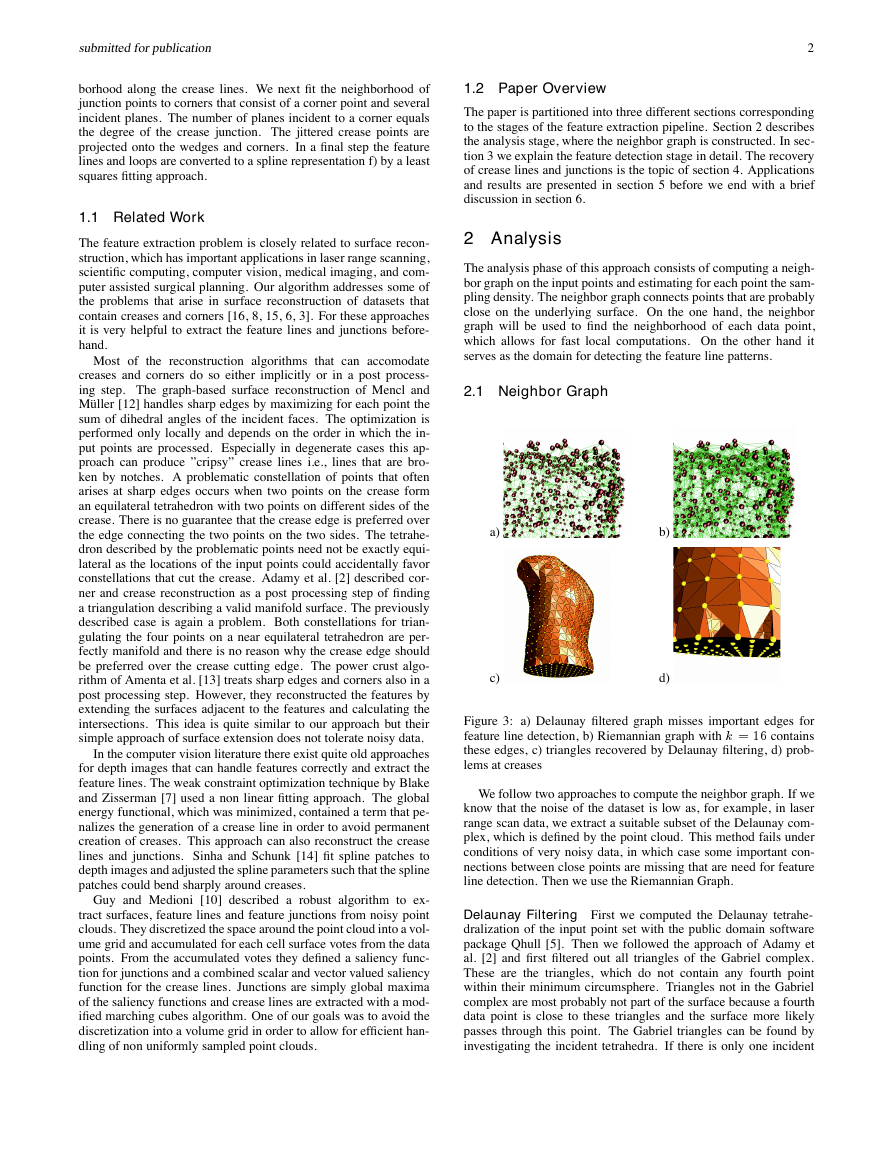
Figure 3: a) Delaunay filtered graph misses important edges for
feature line detection, b) Riemannian graph with k = 16 contains
these edges, c) triangles recovered by Delaunay filtering, d) prob-
lems at creases
We follow two approaches to compute the neighbor graph. If we
know that the noise of the dataset is low as, for example, in laser
range scan data, we extract a suitable subset of the Delaunay com-
plex, which is defined by the point cloud. This method fails under
conditions of very noisy data, in which case some important con-
nections between close points are missing that are need for feature
line detection. Then we use the Riemannian Graph.
Delaunay Filtering First we computed the Delaunay tetrahe-
dralization of the input point set with the public domain software
package Qhull [5]. Then we followed the approach of Adamy et
al. [2] and first filtered out all triangles of the Gabriel complex.
These are the triangles, which do not contain any fourth point
within their minimum circumsphere. Triangles not in the Gabriel
complex are most probably not part of the surface because a fourth
data point is close to these triangles and the surface more likely
passes through this point. The Gabriel triangles can be found by
investigating the incident tetrahedra. If there is only one incident
�
submittedforpublication
3
tetrahedron, we check if the center of its circumsphere is on the
same side of the triangle as the fourth point of the tetrahedron. In
case of two incident tetrahedra, we check if their circumsphere cen-
ters lay on different sides of the triangle.
The second step of the algorithm is to filter out a reasonable sub-
set of the Gabriel complex, which describes the surface. We used
two triangle filters. The first was a simplified version of Adamy
et al.’s umbrella filter, which ensures that the triangles incident on
each data point form at least one closed fan. To find a good guess for
this fan, the Gabriel triangles incident on a point are sorted accord-
ing to a parameter, which gives a reasonable measure of whether the
triangle should be part of the surface. For each data point, triangles
are extracted from the sorted list, until the first fan is completed at
which point these triangles are validated as part of the output of the
filter. We implemented the fan detection and identification with a
modified version of a disjoint set data structure that did not prune
the trees of the connected sets.
The simplified umbrella filter closes the holes of the model and
connects different surface parts (see figure 4 a) and c)). The aim of
the second filter was to recover the holes and to disconnect distant
surface parts simply by eliminating triangles that have extraordinar-
ily long edges. For this, we first computed the average edge length
at each data point. Then we removed all triangles which contained
an edge that was three times longer than the average edge length
of the two incident vertices. In this way we coverered holes and
disconnected nearby but disjoint surface parts (see figure 4 b) and
d)).
The Delaunay filtering has the advantage that it helps to discon-
nect data points that lay on different surface parts. Our simplified
filter did not serve for surface reconstruction, in cases in which the
models contained sharp edges as figures 3 c) and d) illustrate. But
this is not important for our purpose as we detect the creases later
on and only need the neighbor information contained in the pro-
duced triangles. More serious is that the Delaunay filtering does not
produce enough edges (figure 3 a)) for very noisy input data sets,
which causes problems especially for the feature detection stage in
which the output is a subset of the neighbor graph. The two Delau-
nay filters are relatively fast and consumeed for the brain dataset of
figure 13 with 84,000 points about 10 seconds, which is about one
third of the time consumed by Qhull.
Riemannian Graph The Riemannian graph contains for each
data point the edges to the k nearest neighbors, where we chose k
between 10 and 16. For our purposes we could compute a sufficient
approximation to the Riemannian graph with the approximate near-
est neighbor library ANN [4]. For the brain dataset the Riemannian
graph was computed in 7 to 10 seconds for k = 10 to 16. The
advantage of the Riemannian Graph is that it can handle noisy data
and consumes much less time than the Delaunay filtering approach.
2.2 Sampling Density
In the following computations it was often important to relate the
computed quantities to the sampling density. Most often we needed
the sampling density in units of length. Therefore we defined the
average distance i of a data point �i with the set �i of direct
neighbor points in the neighbor graph as
i :
1
j�ij
X
�2�i
j�i � �j
(1)
3 Feature Detection
In this section we describe how to find the crease and border pat-
terns in a point cloud. The first stage analyzes the neighborhood
a)
c)
b)
d)
Figure 4: Effects of filtering long triangles: a) closed holes before
filter, b) holes recovered, c) inter-surface connections before filter,
d) surface separated
of each data point and classifies the points into surface points, po-
tential crease points and potential border points. For the latter two
cases we must determine penalty functions, which measure the un-
likelihood of a data point to be on a crease or a border line.
The second stage extracts the feature line patterns. The edges
of the adjacency graph are weighted with the penalty functions of
their incident data points. We used a modified minimum spanning
tree algorithm to extract the feature line patterns.
3.1 Point Classification
For each data point �i one must gather from the neighbor graph a
set �i of neighbor data points. The number of neighbors collected
depends on the noise level of the dataset. For data with low or no
noise it is necessary only to gather the direct neighbors of the data
points while for highly noisy data one must consider all neighbors
with a graph distance less than three four or five edges depending
on the noise level.
From the set of neighbors we extracted two quantities. The cen-
ter location ci and the correlation matrix Ci given by
�R3 3 ci
�R3�3 3 Ci
def
=
def
=
1
j�ij
1
j�ij
X
�
�2�i
X
�2�i
�� � ci��� � ci��:
(2)
(3)
The eigenvectors fe0; e1; e2g of the correlation matrix together
with the corresponding eigenvalues f0; 1; 2g, where 0
1 2, define the correlation ellipsoid that adopts the general
form of the neighbor points. Figure 5 shows the different shapes,
that we are interested in. It shows in green color the surface type
at the current data point: plane, crease wedge, border half plane
and corner. The data point is the yellow ball and the correlation
ellipsoid is depicted around the centroid ci in violet.
�
submittedforpublication
4
a)
c)
b)
d)
Figure 5: shape of the correlation ellipsoid around different types
of data points: a) surface point, b) crease point, c) border point, d)
corner point
For a point on a flat surface the ellipsoid degenerates to a pancake
with 1 2 and 0 0. The unit vector e0 points in normal
direction, illustrated by the arrow in figure 5 a). The normal dervied
in this way is actually the surface normal of a plane fitted to the set
of neighbors, that minimizes the squared distance to the neighbors.
The optimal plane must go through the centroid ci. The equivalence
of the different normal estimations can be seen easily by looking
briefly at the least squares problem. Suppose ^� is the normal of the
optimal plane. Then we want to minimize ��2�i
�^���� � ci��2
under the constraint ^�� ^� = 1. By the method of the Langrange
multipliers we need to minimize
X
�2�i
^���� � ci��� � ci�� ^� � �1 � ^�� ^�� = ^���Ci � ��^� �
with the Langrange multiplier . Notice that vv� denotes the outer
vector product, which results in a simmetric matrix, whereas v�v
denotes the dot product. Setting the gradient for ^� of this equa-
tion to zero yields exactly the eigenvalue equation Ci ^� = ^�. The
solution with the minimum residual is given by the eigenvector cor-
responding to the smallest eigenvalue.
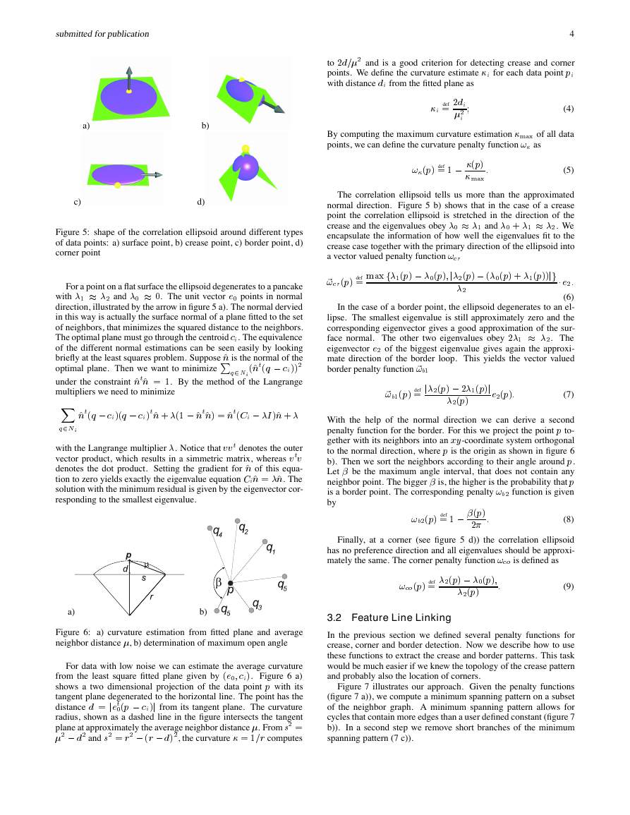
a)
b)
Figure 6: a) curvature estimation from fitted plane and average
neighbor distance , b) determination of maximum open angle
For data with low noise we can estimate the average curvature
from the least square fitted plane given by �e0; ci�. Figure 6 a)
shows a two dimensional projection of the data point � with its
tangent plane degenerated to the horizontal line. The point has the
distance d = je�
0�� � ci�j from its tangent plane. The curvature
radius, shown as a dashed line in the figure intersects the tangent
plane at approximately the average neighbor distance . From �2 =
2 � d2 and �2 = �2 � �� � d�2, the curvature = 1=� computes
to 2d=2 and is a good criterion for detecting crease and corner
points. We define the curvature estimate i for each data point �i
with distance di from the fitted plane as
i
def
=
2di
2
i
;
(4)
By computing the maximum curvature estimation �ax of all data
points, we can define the curvature penalty function ! as
!���
def
= 1 �
���
�ax
:
(5)
The correlation ellipsoid tells us more than the approximated
normal direction. Figure 5 b) shows that in the case of a crease
point the correlation ellipsoid is stretched in the direction of the
crease and the eigenvalues obey 0 1 and 0 � 1 2. We
encapsulate the information of how well the eigenvalues fit to the
crease case together with the primary direction of the ellipsoid into
a vector valued penalty function !c�
def
=
2
~!c����
�axf1��� � 0���;j2��� � �0��� � 1����jg
� e2:
(6)
In the case of a border point, the ellipsoid degenerates to an el-
lipse. The smallest eigenvalue is still approximately zero and the
corresponding eigenvector gives a good approximation of the sur-
face normal. The other two eigenvalues obey 21 2. The
eigenvector e2 of the biggest eigenvalue gives again the approxi-
mate direction of the border loop. This yields the vector valued
border penalty function ~!b1
~!b1���
def
= j2��� � 21���j
2���
e2���:
(7)
With the help of the normal direction we can derive a second
penalty function for the border. For this we project the point � to-
gether with its neighbors into an xy-coordinate system orthogonal
to the normal direction, where � is the origin as shown in figure 6
b). Then we sort the neighbors according to their angle around �.
Let be the maximum angle interval, that does not contain any
neighbor point. The bigger is, the higher is the probability that �
is a border point. The corresponding penalty !b2 function is given
by
!b2���
def
= 1 �
���
2
:
(8)
Finally, at a corner (see figure 5 d)) the correlation ellipsoid
has no preference direction and all eigenvalues should be approxi-
mately the same. The corner penalty function !c� is defined as
!c����
def
=
2��� � 0���;
2���
:
(9)
3.2 Feature Line Linking
In the previous section we defined several penalty functions for
crease, corner and border detection. Now we describe how to use
these functions to extract the crease and border patterns. This task
would be much easier if we knew the topology of the crease pattern
and probably also the location of corners.
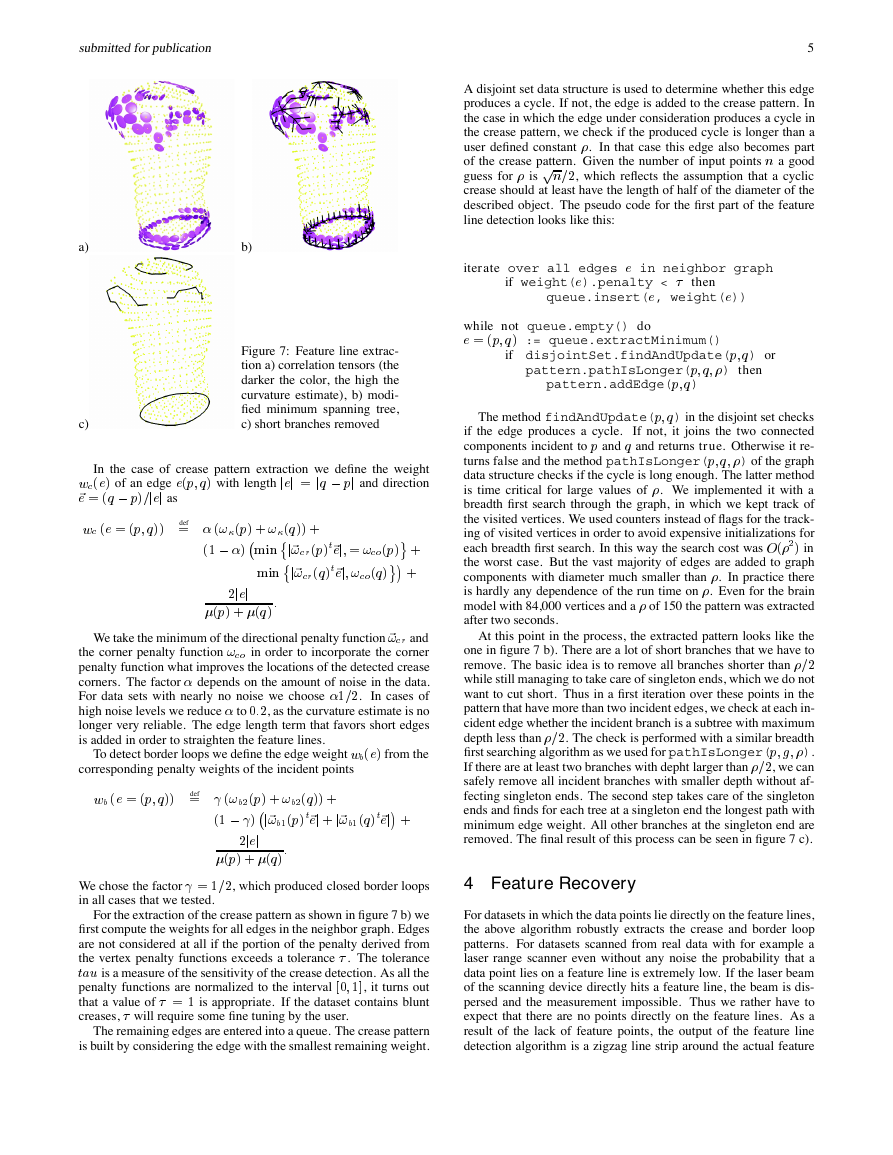
Figure 7 illustrates our approach. Given the penalty functions
(figure 7 a)), we compute a minimum spanning pattern on a subset
of the neighbor graph. A minimum spanning pattern allows for
cycles that contain more edges than a user defined constant (figure 7
b)). In a second step we remove short branches of the minimum
spanning pattern (7 c)).
�
submittedforpublication
5
A disjoint set data structure is used to determine whether this edge
produces a cycle. If not, the edge is added to the crease pattern. In
the case in which the edge under consideration produces a cycle in
the crease pattern, we check if the produced cycle is longer than a
user defined constant . In that case this edge also becomes part
of the crease pattern. Given the number of input points � a good
guess for is ��=2, which reflects the assumption that a cyclic
crease should at least have the length of half of the diameter of the
described object. The pseudo code for the first part of the feature
line detection looks like this:
a)
c)
b)
Figure 7: Feature line extrac-
tion a) correlation tensors (the
darker the color, the high the
curvature estimate), b) modi-
fied minimum spanning tree,
c) short branches removed
In the case of crease pattern extraction we define the weight
wc�e� of an edge e��; �� with length jej = j� � �j and direction
~e = �� � ��=jej as
wc �e = ��; ���
def
= �!��� � !���� �
�1 � � ��i� �j~!c�����~ej; = !c���� �
�i��j~!c�����~ej; !c���� � �
2jej
:
��� � ���
We take the minimum of the directional penalty function ~!c� and
the corner penalty function !c� in order to incorporate the corner
penalty function what improves the locations of the detected crease
corners. The factor depends on the amount of noise in the data.
For data sets with nearly no noise we choose 1=2.
In cases of
high noise levels we reduce to 0:2, as the curvature estimate is no
longer very reliable. The edge length term that favors short edges
is added in order to straighten the feature lines.
To detect border loops we define the edge weight wb�e� from the
corresponding penalty weights of the incident points
wb �e = ��; ���
def
= �!b2��� � !b2���� �
�1 � � �j~!b1����~ej � j~!b1����~ej� �
2jej
:
��� � ���
We chose the factor = 1=2, which produced closed border loops
in all cases that we tested.
For the extraction of the crease pattern as shown in figure 7 b) we
first compute the weights for all edges in the neighbor graph. Edges
are not considered at all if the portion of the penalty derived from
the vertex penalty functions exceeds a tolerance . The tolerance
�a is a measure of the sensitivity of the crease detection. As all the
penalty functions are normalized to the interval [0; 1], it turns out
that a value of = 1 is appropriate. If the dataset contains blunt
creases, will require some fine tuning by the user.
The remaining edges are entered into a queue. The crease pattern
is built by considering the edge with the smallest remaining weight.
iterate over all edges e in neighbor graph
if weight(e).penalty < then
queue.insert(e, weight(e))
while not queue.empty() do
e = ��; �� := queue.extractMinimum()
if disjointSet.findAndUpdate(�; �) or
pattern.pathIsLonger(�; �; ) then
pattern.addEdge(�; �)
The method findAndUpdate(�; �) in the disjoint set checks
if the edge produces a cycle.
If not, it joins the two connected
components incident to � and � and returns true. Otherwise it re-
turns false and the method pathIsLonger(�; �; ) of the graph
data structure checks if the cycle is long enough. The latter method
is time critical for large values of . We implemented it with a
breadth first search through the graph, in which we kept track of
the visited vertices. We used counters instead of flags for the track-
ing of visited vertices in order to avoid expensive initializations for
each breadth first search. In this way the search cost was ��2� in
the worst case. But the vast majority of edges are added to graph
components with diameter much smaller than . In practice there
is hardly any dependence of the run time on . Even for the brain
model with 84,000 vertices and a of 150 the pattern was extracted
after two seconds.
At this point in the process, the extracted pattern looks like the
one in figure 7 b). There are a lot of short branches that we have to
remove. The basic idea is to remove all branches shorter than =2
while still managing to take care of singleton ends, which we do not
want to cut short. Thus in a first iteration over these points in the
pattern that have more than two incident edges, we check at each in-
cident edge whether the incident branch is a subtree with maximum
depth less than =2. The check is performed with a similar breadth
first searching algorithm as we used for pathIsLonger(�; g; ).
If there are at least two branches with depht larger than =2, we can
safely remove all incident branches with smaller depth without af-
fecting singleton ends. The second step takes care of the singleton
ends and finds for each tree at a singleton end the longest path with
minimum edge weight. All other branches at the singleton end are
removed. The final result of this process can be seen in figure 7 c).
4 Feature Recovery
For datasets in which the data points lie directly on the feature lines,
the above algorithm robustly extracts the crease and border loop
patterns. For datasets scanned from real data with for example a
laser range scanner even without any noise the probability that a
data point lies on a feature line is extremely low. If the laser beam
of the scanning device directly hits a feature line, the beam is dis-
persed and the measurement impossible. Thus we rather have to
expect that there are no points directly on the feature lines. As a
result of the lack of feature points, the output of the feature line
detection algorithm is a zigzag line strip around the actual feature
�
submittedforpublication
6
defined by two planes �1 and �2. The dotted line shows how the
wedge splits the space into three regions A; B and C. All points
in region A are closest to plane �1, the ones in region B to �2, and
the points in region C are closest to the intersection line (or in two
dimensions, the intersection point) of the two planes. This split into
three regions makes a least squares fitting approach extremely dif-
ficult, as it is not known in advance which point will fall into which
region after the fitting process. Thus the primary question is how to
split the input points into regions.
The approach described in the next subsection splits the diffi-
cult three-dimensional problem into a number of simplified two-
dimensional problems, where the grouping problem can be solved
efficiently. A robust approximate solution to the three-dimensional
grouping problem is then composed from the two-dimensional so-
lutions via a voting process. In this way we can exploit the infor-
mation available from the feature detection stage to simplify the
feature recovery. After we have derived a reliable grouping we can
fit the wedges to the points in the crease neighborhood and project
the potential crease points directly onto the crease.
This crease line recovery approach breaks down close to crease
junctions as too many data points are incorporated into the fit-
ting process. For this reason we first determine the point group-
ing around corners. As we exploit the solution strategy of the line
recovery but in a more complicated manner, we describe the line
recovery process first.
a)
c)
b)
d)
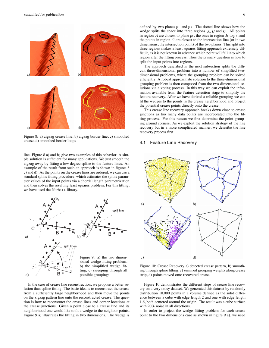
Figure 8: a) zigzag crease line, b) zigzag border line, c) smoothed
crease, d) smoothed border loops
4.1 Feature Line Recovery
line. Figure 8 a) and b) give two examples of this behavior. A sim-
ple solution is sufficient for many applications. We just smooth the
zigzag away by fitting a low degree spline to the feature lines. An
example of the result from such an approach is shown in figures 8
c) and d). As the points on the crease lines are ordered, we can use a
standard spline fitting procedure, which estimates the spline param-
eter values of the input points via a chordal length parametrization
and then solves the resulting least squares problem. For this fitting,
we have used the Nurbs++ library.
a)
c)
b)
Figure 9: a) the two dimen-
sional wedge fitting problem,
b) the simplified wedge fit-
ting, c) sweeping through all
possible groupings
a)
c)
b)
d)
Figure 10: Crease Recovery a) detected crease pattern, b) smooth-
ing through spline fitting, c) summed grouping weights along crease
strip, d) points moved onto recovered crease
In the case of crease line reconstruction, we propose a better so-
lution than spline fitting. The basic idea is to reconstruct the crease
from a sufficiently large neighborhood and then move the points
on the zigzag pattern line onto the reconstructed crease. The ques-
tion is how to reconstruct the crease lines and corner locations at
the crease junctions. Given a point close to a crease line and its
neighborhood one would like to fit a wedge to the neighbor points.
Figure 9 a) illustrates the fitting in two dimensions. The wedge is
Figure 10 demonstrates the different steps of crease line recov-
ery on a very noisy dataset. We generated this dataset by randomly
distribution 10,000 points in a volume defined as the solid differ-
ence between a cube with edge length 2 and one with edge length
1.6, both centered around the origin. The result was a cube surface
with 20% noise in all directions.
In order to project the wedge fitting problem for each crease
point to the two dimensions case as shown in figure 9 a), we need
�
submittedforpublication
7
to know the crease direction or a good approximation to it. As the
detected feature lines are noisy, we use the spline approximation.
From the spline fitting process we know for each crease point, �,
the parameter value �� of its counterpart on the spline ����. Thus
def
= ����� and crease di-
we can compute the smoothed location ��
= _�����=j _�����j. We extend d� to an orthogonal coordi-
rection d�
nate system with an xy plane orthogonal to d� and project neighbor
points of � to the xy plane arriving at the configuration described
in figure 9 b).
def
The wedge fitting problem in two dimensions is still very diffi-
cult as we do not know the zenith location of the wedge. Thus we
simplify the problem be assuming that �� is the zenith of the wedge.
Furthermore we split the space at the split line into only two regions
A and B, as depicted in figure 9 b). The distances from the points
in the previously defined region C to the wedge are underestimated
(see neighbors �A and �B in figure 9 b) for two examples). This
is not a serious problem for our application as these points are rare
and their existance either implies that we detected the crease point
wrong or that there is noise in the data.
The helpful property of the simplified wedge fitting problem is
that no matter what the solution is, the points are split into two
groups at a split line that goes through ��. There are only � of these
groupings, where � is the number of points in the neighborhood.
We can enumerate them by sweeping the split line in a rotational
motion through the neighbor points as illustrated in figure 9 c). The
final solution is the one with the smallest residual.
Given the set of neighbor points � and a grouping �1 _\�2 =
�, the solution of the simplified wedge fitting problem is found by
solving two least square line fitting problems. To each neighbor
group �1 and �2 we fit a line through the origin ��. To avoid the
���� floating point operations per grouping, we prepare the input
matrices
�R2�2 3 �j
def
= X
���
�2�j
j 2 f1; 2g
incrementally during the rotation of the split line. For the first split
line location we compute the matrices explicitly. Each time the
split line rotates one step further, only one point � changes from
one group to the next. We subtract ��� from the matrix of the group
that � leaves and add it to the other matrix. As the matrices are
symmetric and we are in two dimensions, the cost is only three
multiplications and six additions. Given the matrix �i, the normal
to the optimal line is given by the eigenvector of �i correspond-
ing to the smallest eigenvalue. The following algorithm computes
this eigenvector of a matrix � with three square root operations,
one division, four multiplications, five additions and some sign and
binary shift operations.
a := ��11 � �22�=2;
if a = 0 and �12 = 0 then return �1; 0�
if �12 = 0 then
if a > 0 then return �0; 1�
else return �1; 0�
if a = 0 then
if �12 > 0 then return ��2; ��2�=2
else return ��2; �2�=2
12�
f := a=�2�a2 � �2
c := �1=2 � f
d := �g���12��1=2 � f
if �g��a� = �g��d2 � c2� then return �c; d�
else return �d; �c�
Now we are in the position to efficiently group the neighbor-
hoods of each crease point optimally according to the simplified
wedge fitting problem. However, each single grouping might con-
tain a few misgrouped data points, for example if the crease has
a sharp turn. We want to combine as many groupings of adjacent
crease points as possible. The maximum subgraph of a crease pat-
tern, where the neighboring points split into exactly two groups, is
either a closed loop or a path connecting two crease points of degree
unequal two, i.e. crease junctions and singleton ends. We call these
maximum crease paths crease strips. For each crease strip we attach
a weight field to each of the data point that is adjacent to at least one
point on the crease strip. After inititalizing the weights to zero, we
start a voting process at one end of the strip. We build the xy coordi-
nate system orthogonal to the spline direction and find the optimal
grouping of the neighbors that solves the simplified wedge fitting
problem. The weights of neighbors are incremented for members
of group A and decremented for group B members. The amount of
the increment decreases with increasing distance from the wedge
zenith. When we move on to the next crease point on the strip,
we choose x- and y-axes as close as possible to the previous axes,
such that we can identify the groups A and B of the new grouping
with the previous groups. In this way we sweep through the strip
and increment and decrement weights for the neighbors. A sample
weighting along one crease strip in the cube model is shown in fig-
ure 10 c). After all crease points have contributed to the weights,
we classify the neighbor points into group A if their final weight is
positive and into group B if the resulting weight is negative. If a
weight is very close to zero we do not consider the corresponding
neighbor point in the final recovery stage.
In the end we derive a grouping of the crease neighbors that ex-
ploits all the information we get from the feature detection stage. A
final iteration through the points on the crease strip recovers the ori-
gin crease locations. The neighborhood of each point on the strip
is now reliably split into two groups. Thus we can fit two planes
to the two groups in the least square sense by computing and ana-
lyzing the correlation matrix for each group relative to the centroid
of the group. The local crease approximation is the intersection of
the resulting planes. We project the crease point orthogonally onto
the crease approximation. Figure 10 d) shows the result, a more
or less straight line for the cube dataset with 20% noise. There
are still problems near the crease junctions because we do not ex-
clude neighbors in opposite faces of the creases. The solution to
this problem is described in the next section.
4.2 Feature Junction Recovery
In order to find realistic crease lines and their intersection at crease
line junctions, we have to solve the corner fitting problem. Suppose
we have a junction of k intersecting crease lines. The surface is
split into k regions, which are planar near the junction as depicted
in figure 11 a). The corner, which we want to fit to the data points,
is given by the piecewise planar approximation of the surface at
the junction. It is defined by the corner point and k plane normals.
For a least squares fit of a corner to a set of data points we have
to split the data points into k groups, such that the total residual
of square distances is minimized, when k planes are fit to the k
groups. Figure 11 c) shows such a grouping. This problem is more
difficult than the wedge fitting problem and the number of different
groupings increases exponentially with k, even if we can arrange
the vertices in a linear order.
Figure 11 illustrates our approach to an approximate solution of
the corner fitting problem. Suppose we start of with a crease junc-
tion point �c detected in the feature detection stage. First we find
a two dimensional projection of the problem, in which the points
in the neighborhood �c of �c can be sorted around �c according to
their angle relative to an arbitrary x-axis in the projected space (fig-
ure 11 b)). We can imagine different approaches to do this. First
we could fit an ellipsoid to the point set [1] and use the direction
�
submittedforpublication
8
the grouping terminated after two or three iterations.
Given the optimal grouping, we can fit k planes to each of the
k groups and reconstruct the corner. For k > 3 the planes do not
always intersect in a single point. Therefore, we again use a least
squares approach to reconstruct the corner location. We minimize
the square distance to all of the k planes. The tool to solve this min-
imization problem is also known as quadric error metrics, orignally
introduced by Garland [9] in mesh simplification to find optimal lo-
cations for the mesh vertice after an edge collapse operation. With
the knowledge of the vertex grouping around the junction point, we
can finally recover the crease close to the junction by not consider-
ing any of the data points of �c that do not belong to the two groups
of the crease strip.
Let us summarize. The feature recovery stage first groups the
neighborhoods around crease junctions into as many groups as there
are incident faces. From the grouping the corner locations are re-
covered. Then the crease lines close to the junctions are recon-
structed with the knowledge about grouping near the junctions. Fi-
nally, the remaining parts of the crease lines are recovered with the
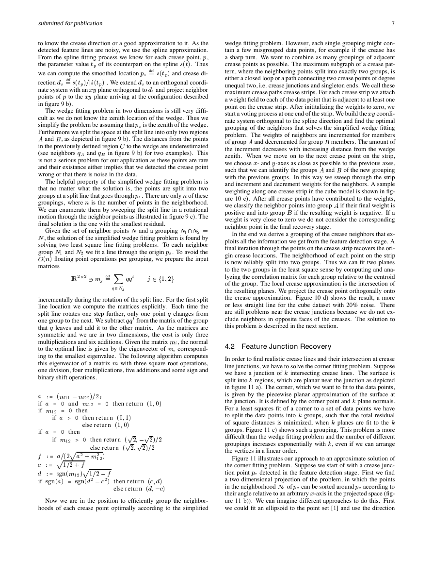
method described in the previous section. Figure 11 f) shows the
final result of the noisy cube.
5 Applications & Results
5.1 Surface Meshing
Our primary goal in developing the feature extraction algorithm was
as the first stage of a point cloud mesh generation tool. The basic
idea behind the point cloud mesh generator is to locally fit polyno-
mial patches to the point cloud and directly generate a mesh with
element sizes that are adapted to curvature and to an anisotropic siz-
ing function. The mesh is generated with an advancing front algo-
rithm. While the front advances a new local approximation is com-
puted, whenever the front leaves the domain of the current polyno-
mial patch. An important ingredient is again a neighbor graph that
reflects the proximity along the surface. Problems arise as always at
the crease lines, where a naively computed neighbor graph connects
the different surface parts incident to the crease. This will dimin-
ish the quality of the fitted patch near the crease lines significantly.
With the help of point grouping along the edges, as described in sec-
tion 4.1 and 4.2, we can easily remove all edges that cut the creases
and corners. Thus our feature extraction stage not only produces
the feature lines for the point cloud mesher, but also a sophisticated
neighbor graph.
5.2 Point Cloud Enrichment
a)
b)
c)
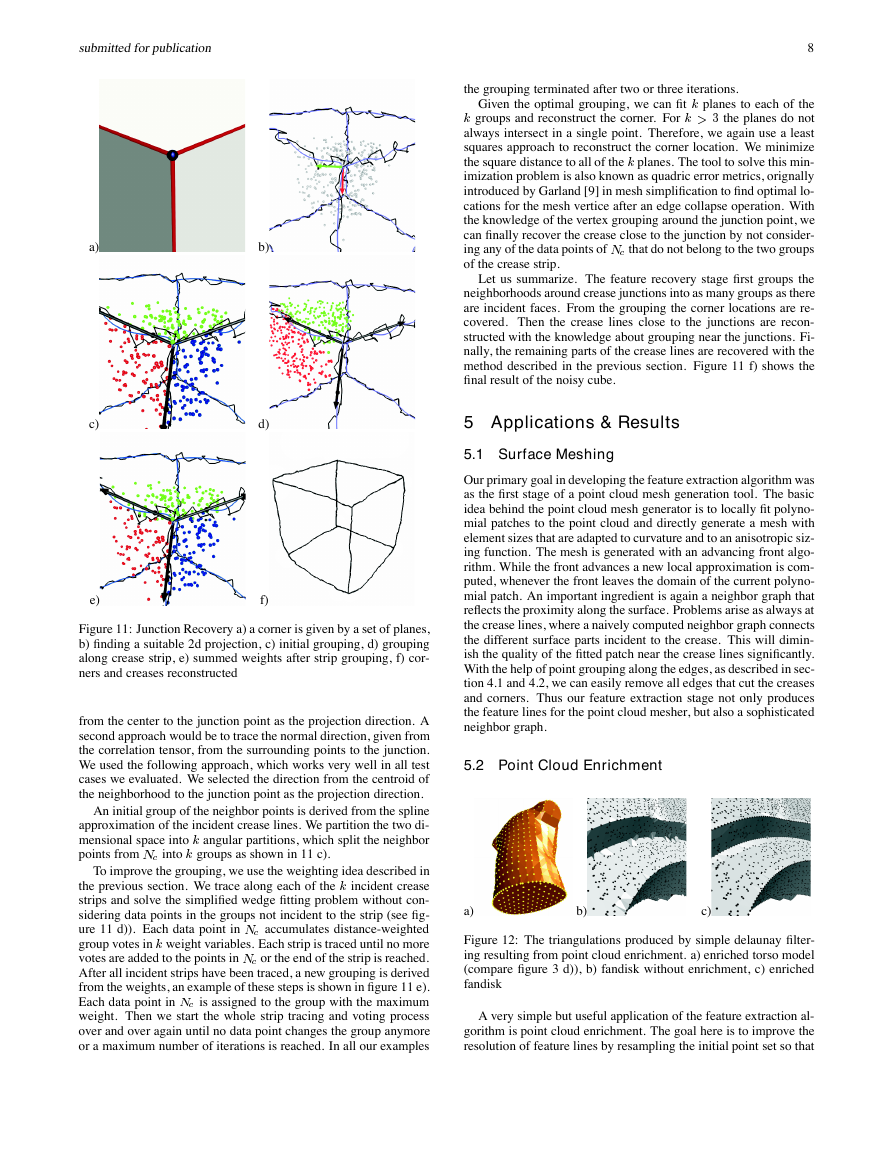
Figure 12: The triangulations produced by simple delaunay filter-
ing resulting from point cloud enrichment. a) enriched torso model
(compare figure 3 d)), b) fandisk without enrichment, c) enriched
fandisk
A very simple but useful application of the feature extraction al-
gorithm is point cloud enrichment. The goal here is to improve the
resolution of feature lines by resampling the initial point set so that
a)
c)
e)
b)
d)
f)
Figure 11: Junction Recovery a) a corner is given by a set of planes,
b) finding a suitable 2d projection, c) initial grouping, d) grouping
along crease strip, e) summed weights after strip grouping, f) cor-
ners and creases reconstructed
from the center to the junction point as the projection direction. A
second approach would be to trace the normal direction, given from
the correlation tensor, from the surrounding points to the junction.
We used the following approach, which works very well in all test
cases we evaluated. We selected the direction from the centroid of
the neighborhood to the junction point as the projection direction.
An initial group of the neighbor points is derived from the spline
approximation of the incident crease lines. We partition the two di-
mensional space into k angular partitions, which split the neighbor
points from �c into k groups as shown in 11 c).
To improve the grouping, we use the weighting idea described in
the previous section. We trace along each of the k incident crease
strips and solve the simplified wedge fitting problem without con-
sidering data points in the groups not incident to the strip (see fig-
ure 11 d)). Each data point in �c accumulates distance-weighted
group votes in k weight variables. Each strip is traced until no more
votes are added to the points in �c or the end of the strip is reached.
After all incident strips have been traced, a new grouping is derived
from the weights, an example of these steps is shown in figure 11 e).
Each data point in �c is assigned to the group with the maximum
weight. Then we start the whole strip tracing and voting process
over and over again until no data point changes the group anymore
or a maximum number of iterations is reached. In all our examples
�




 2023年江西萍乡中考道德与法治真题及答案.doc
 2012年重庆南川中考生物真题及答案.doc
 2013年江西师范大学地理学综合及文艺理论基础考研真题.doc
 2020年四川甘孜小升初语文真题及答案I卷.doc
 2020年注册岩土工程师专业基础考试真题及答案.doc
 2023-2024学年福建省厦门市九年级上学期数学月考试题及答案.doc
 2021-2022学年辽宁省沈阳市大东区九年级上学期语文期末试题及答案.doc
 2022-2023学年北京东城区初三第一学期物理期末试卷及答案.doc
 2018上半年江西教师资格初中地理学科知识与教学能力真题及答案.doc
 2012年河北国家公务员申论考试真题及答案-省级.doc
 2020-2021学年江苏省扬州市江都区邵樊片九年级上学期数学第一次质量检测试题及答案.doc
 2022下半年黑龙江教师资格证中学综合素质真题及答案.doc