数据网络答案.pdf-资料库

skyscraper1234-4911036-4744302543307296160.pdf-第1页.png

第1页 / 共70页

skyscraper1234-4911036-4744302543307296160.pdf-第2页.png

第2页 / 共70页

skyscraper1234-4911036-4744302543307296160.pdf-第3页.png

第3页 / 共70页

skyscraper1234-4911036-4744302543307296160.pdf-第4页.png

第4页 / 共70页

skyscraper1234-4911036-4744302543307296160.pdf-第5页.png

第5页 / 共70页

skyscraper1234-4911036-4744302543307296160.pdf-第6页.png

第6页 / 共70页

skyscraper1234-4911036-4744302543307296160.pdf-第7页.png

第7页 / 共70页

skyscraper1234-4911036-4744302543307296160.pdf-第8页.png

第8页 / 共70页

SOLUTIONS MANUAL Second Edition Data Networks DIMITRI BERTSEKAS Massachusetts Institute a/Technology ROBERT GALLAGER Massachusetts Institute a/Technology IIPRENTICE HALL. Englewood Cliffs. New Jersey 07632

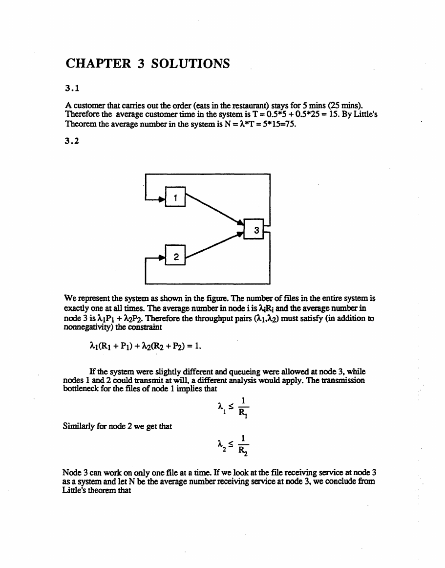
CHAPTER 3 SOLUTIONS 3.1 A customer that carries out the order (eats in the restaurant) stays for 5 mins (25 mins). Therefore the average customer time in the system is T = 0.5*5 + 0.5*25 = 15. By Little's Theorem the average number in the system is N = A*T =5*15=75. 3.2 We represent the system as shown in the figure. The number of fl1es in the entire system is exactly one at all times. The average number in node i is AiRi and the average number in node 3 is'IolPl + A2P2. Therefore the throughput pairs (AhA2) must satisfy (in addition to nonnegativity) the constraint If the system were slightly different and queueing were allowed at node 3, while nodes 1 and 2 could transmit at will, a different analysis would apply. The transmission bottleneck for the files of node 1 implies that Similarly for node 2 we get that 1 A S - } R} Node 3 can work on only one file at a time. If we look at the flle receiving service at node 3 as a system and let N be the average number receiving service at node 3, we conclude from Little's theorem that

and N S 1 This implies that AIPI + A P2 S 1 2 3.3 Working Machines ...-. R Machines .Waiting Repair Q Repairmen We represent the system as shown in the figure. In particular, once a machine breaks down, it goes into repair if a repairperson is available at the time, and otherwise waits in a queue for a repaiIperson to become free. Note that ifm=1 this system is identical to the one of Example 3.7. Let Abe the throughput of the system and let Q be the average time a broken down machine waits for a repairperson to become free. Applying Little's theorem to the entire system, we obtain A(R+Q+P) =N from which A(R+P) S N (1) (2) Since the number of machines waiting repair can be at most (N-m), the average waiting time AQ is at most the average time to repair (N-m) machines, which is (N-m)P. Thus, from Eq. (1) we obtain A(R+ (N - m)P + P) ~ N Applying Little's theorem to the repairpersons, we obtain APSm (3) (4)

The relations (2)-(4) give the following bounds for the throughput A '1 < . {m N } R + (N - m +1)P ~ I\. - nun p 'R + P N ..... (5) Note that these bounds generalize the ones obtained n Example 3.7 (see Eq. (3.9». By using the equation T=N/A. for the average time between repairs, we obtain from Eq. 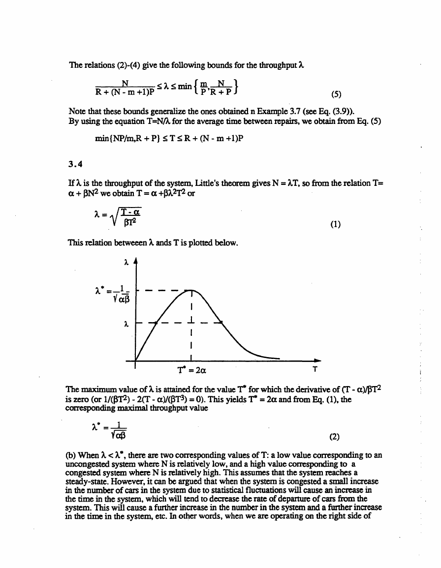(5) min{NP/m,R + P} S; T S; R + (N - m +1)P 3.4 IfAis the throughput of the system, Little's theorem gives N = AT, so from the relation T= a + J3N2 we obtain T = a +J3A.2T2 or A=VTrr; (1) This relation betweeen A. ands T is plotted below. ~=2a T The maximum value of A. is attained for the value 1"" for which the derivative of (T - a)/J3T2 is zero (or 1/(131'2) - 2(T - a)/(J3T3) = 0). This yields 1"" = 2a and from Eq. (1), the corresponding maximal throughput value A* =_1_vap (2) (b) When A. < A.", there are two corresponding values of T: a low value corresponding to an uncongested system where N is relatively low, and a high value corresponding to a congested system where N is relatively high. This assumes that the system reaches a steady-state. However, it can be argued that when the system is congested a small increase in the number of cars in the system due to statistical fluctuations will cause an increase in the time in the system, which will tend to decrease the rate of departure of cars from the system. This will cause a further increase in the number in the system and a funher increase in the time in the system, etc. In other words, when we are operating on the right side of

the curve of the figure, there is a tendency for instability in the system, whereby a steady state is never reached: the system tends to drift towards a traffic jam where the car depature rat~ from the system tends towards zero and the time a car spends in the system tends towards infinity. Phenomena of this type are analyzed in the context of the Aloha multiaccess system in Chapter 4. 3.5 The expected time in question equals E{Time} = (5 + E{stay of 2nd student})*P{ 1st stays less or equal to 5 minutes} + (E(stayof 1st Istay of 1st ~ 5} + E{stay of2nd})* . P{1st stays more than 5 minutes}. We have E(stay of 2nd student} = 30, and, using the memoryless property of the exponential distribution, E{stay of 1st I stay of lst ~ 5} = 5 + E(stay of 1st} = 35. Also P {1st student stays less or equal to 5 minutes} = 1 - e-S/30 P {1st student stays more than 5 minutes} = e-S/3o. By substitution we obtain E{Time} = (5 + 30)*(1 - e-S/3o) + (35 + 30)* e-SI3O =35 + 30*e-SI30 = 60.394. 3.6 (a) The probability that the person will be the last to leave is 1/4 because the exponential distribution is memoryless, and all customers have identical service time distribution. In particular, at the instant the customer enters service, the remaining service time of each of the other three customers served has the same distribution as the service time of the customer. (b) The average time in the bank is 1 (the average customer service time) plus the expected time for the first customer to finish service. The latter time is 1/4 since the departure process is statistically identical to that of a single server facility with 4 times larger service rate. More precisely we have P {no customer departs in the next t mins} =P {I st does not depart in next t mins} * P{2nd does not depart in next t mins} * P{ 3rd does not depart in next t mins} * P{4th does not depart in next t mins} = (e-t)4 = e-4t. Therefore P(the first departure occurs within the nextt mins} = I - e-4t,

and the expected time to the next depature is 1/4. So the answer is 5/4 minutes. (c) The answer will not change because the situation at the instant when the customer begins service will be the same under the conditions for (a) and the conditions for (c). 3.7 In the statistical multiplexing case the packets of at most one of the streams will wait upon arrival for a packet of the other stream to finish transmission. Let W be the waiting time , and note that 0 ~ W ~ T/2. We have that one half of the packets have system time T/2 + W and waiting time in queue W. Therefore Average System Time = (l/2)T/2 + (1/2)(T/2+W) = (T+W)/2 Average Waiting Time in Queue =W/2 Variance of Waiting Time = (1/2)(W/2)4(l/2)(W/2)2 = W2/4. So the average system time is between T/2 and 3T/4 and the variance of waiting time is between 0 and T2/16. 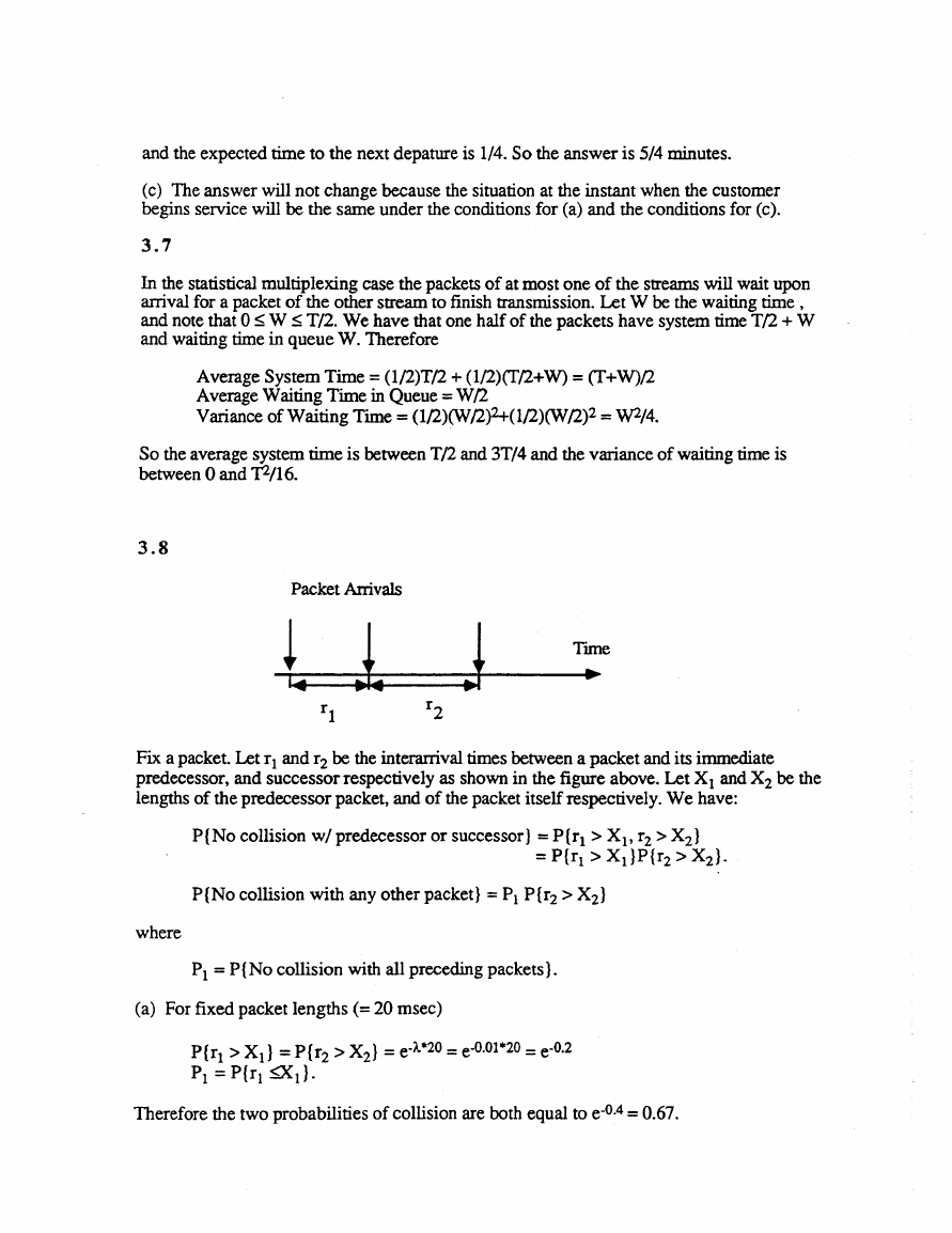3.8 Packet Arrivals ~ 1 J Time • r Z I~ r 1 Fix a packet. Let rl and r2 be the interarrival times between a packet and its immediate predecessor, and successor respectively as shown in the figure above. Let Xl and X2 be the lengths of the predecessor packet, and of the packet itself respectively. We have: P{No collision wi predecessor or successor) = P{rl > Xl' r2 > X2} = P{rl > Xd P {r2 > X2}· P{No collision with any other packet} = PI P{r2 > X2} where PI = P{No collision with all preceding packets}. (a) For fixed packet lengths (= 20 msec) P{rl > Xtl = P{r2 > X2} =e-I..*20 =e-O.OI*20 =e-O.2 PI = P{rl ~tl· Therefore the two probabilities of collision are both equal to e-O.4 = 0.67.

(b) For X exponentially distributed packet length with mean 1/1J. we have P{rl > Xl} = P{rz .... >~} =f P{rl > X I Xl = X}p{XI = X}dX o .... o =f e-AXJJe-JiXdX =....JL. A+Jl Substituting A= 0.01 and IJ.= 0.05 we obtain P{rl > Xl} = P{rz > Xz}= 5/6, and P{No collision w/ predecessor or successor} =(5/6)2 = 0.694. Also PI is seen to be the steady-state probability of a customer finding an empty system in the M/MIoo system with arrival and service rate Aand J.1 respectively. Therefore PI =e-AIJI. = e~~.Therefare . P{No collision with any other packet} = e~~5/6 =0.682. 3.9 (a) For each session the arrival rate is A= 150/60 = 2.5 packets/sec. When the line is divided into 10 lines of capacity 5 Kbits/sec, the average packet transmission time is 1/1J.= 0.2 secs. The corresponding utilization factor is p =A/IJ. = 0.5. We have for each session NQ = p2/(l- p) =05, N = p/(1- p) = I, and T =NIA. = 0.4 secs. For all sessions collectively NQ and N must be multiplied by 10 to give NQ = 5 and N = 10. When statistical multiplexing is used, all sessions are merged into a single session with 10 times larger A and J.1.; A= 25, 1I1J. = 0.02. We obtain p = 0.5, NQ = 0.5, N = I, and T = 0.04 secs. Therefore NQt N, and T have been reduced by a factor of 10 over the TOM case. (b) For the sessions transmitting at 250 packets/min we have p = (250/60)*0.2 = 0.833 and we have NQ =(0.833)2/(1 - 0.833) =4.158, N =5, T = Nf).. = 5/(250/60) = 1.197 . ·secs. For the sessions transmitting at 50 packetslmiJi we have p = (50/60)*0.2 =0.166, NQ = 0.033, N = 0.199, T = 0.199/(50/60) =0.239. The corresponding averages over all sessions are NQ = 5*(4.158 + 0.033) = 21, N =5*(5 +0.199) =26, T = Nf).. = N/(5*AI+ 5*A.z) =26/(5*(250/60)+5*(50/60» =1.038 sees. When statistical multiplexing is used the arrival rate of the combined session is 5*(250+ 50) =1500 packets/sec and the same values for NQ, N, and T as in (a) are obtained. 3.10

资料库

数据网络答案.pdf

相关推荐

行业

热门标签

最新资料