SLIC Superpixels
Radhakrishna Achanta, Appu Shaji, Kevin Smith, Aurelien Lucchi,
Pascal Fua, and Sabine S¨usstrunk
School of Computer and Communication Sciences (IC)
´Ecole Polytechnique F´edrale de Lausanne (EPFL)
Abstract. Superpixels are becoming increasingly popular for use in
computer vision applications. However, there are few algorithms that
output a desired number of regular, compact superpixels with a low com-
putational overhead. We introduce a novel algorithm that clusters pixels
in the combined five-dimensional color and image plane space to effi-
ciently generate compact, nearly uniform superpixels. The simplicity of
our approach makes it extremely easy to use – a lone parameter specifies
the number of superpixels – and the efficiency of the algorithm makes it
very practical. Experiments show that our approach produces superpix-
els at a lower computational cost while achieving a segmentation quality
equal to or greater than four state-of-the-art methods, as measured by
boundary recall and under-segmentation error. We also demonstrate the
benefits of our superpixel approach in contrast to existing methods for
two tasks in which superpixels have already been shown to increase per-
formance over pixel-based methods.
1
Introduction
Superpixels provide a convenient primitive from which to compute local im-
age features. They capture redundancy in the image [1] and greatly reduce the
complexity of subsequent image processing tasks. They have proved increasingly
useful for applications such as depth estimation [2], image segmentation [3, 4],
skeletonization [5], body model estimation [6], and object localization [7].
For superpixels to be useful they must be fast, easy to use, and produce high
quality segmentations. Unfortunately, most state-of-the-art superpixel methods
do not meet all these requirements. As we will demonstrate, they often suffer
from a high computational cost, poor quality segmentation, inconsistent size and
shape, or contain multiple difficult-to-tune parameters.
The approach we advocate in this work, while strikingly simple, addresses
these issues and produces high quality, compact, nearly uniform superpixels more
efficiently than state-of-the-art methods [8, 9, 5, 10]. The algorithm we propose,
simple linear iterative clustering (SLIC) performs a local clustering of pixels
in the 5-D space defined by the L, a, b values of the CIELAB color space and
Please cite this paper as: Radhakrishna Achanta, Appu Shaji, Kevin Smith, Aure-
lien Lucchi, Pascal Fua, and Sabine S¨usstrunk, SLIC Superpixels, EPFL Technical
Report 149300, June 2010.
�
2
Achanta et al.
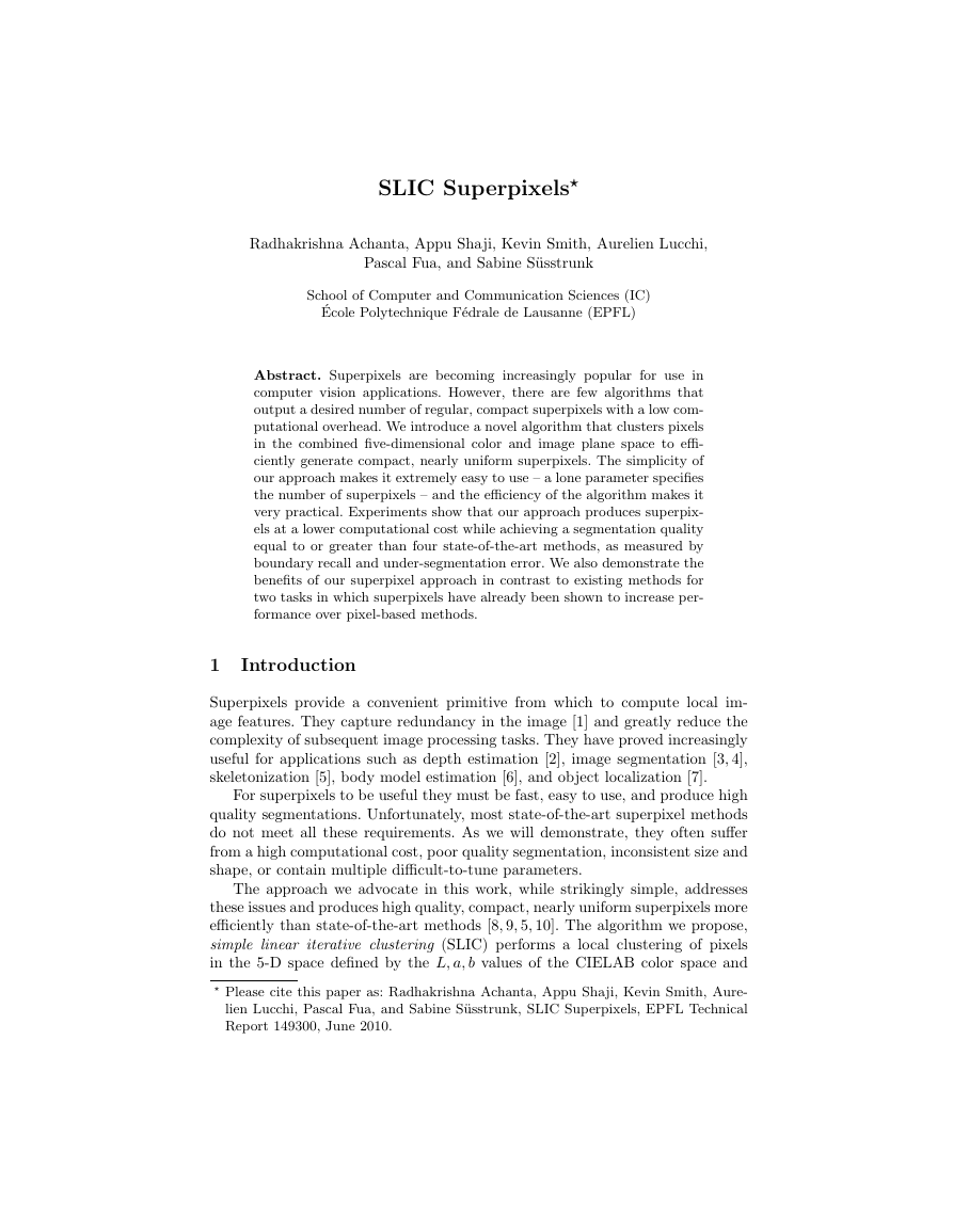
Fig. 1. Image segmented using our algorithm into superpixels of (approximate) size 64,
256, and 1024 pixels. The superpixels are compact, uniform in size, and adhere well to
region boundaries.
the x, y pixel coordinates. A novel distance measure enforces compactness and
regularity in the superpixel shapes, and seamlessly accomodates grayscale as
well as color images. SLIC is simple to implement and easily applied in practice
– the only parameter specifies the desired number of superpixels. Experiments
on the Berkeley benchmark dataset [11] show that SLIC is significantly more
efficient than competing methods, while producing segmentations of similar or
better quality as measured by standard boundary recall and under-segmentation
error measures.
For many vision tasks, compact and highly uniform superpixels that respect
image boundaries, such as those generated by SLIC in Fig. 1, are desirable. For
instance, graph-based models such as Conditional Random Fields (CRF) can see
dramatic speed increases when switching from pixel-based graphs to superpix-
els [3, 7], but loose or irregular superpixels can degrade the performance. Local
features such as SIFT extracted from the image at superpixel locations become
less meaningful and discriminative if the superpixels are loose or irregular, and
learning statistics over cliques of two or more superpixels can be unreliable.
This effect can be seen when we compare the performance of SLIC superpixels
to competing methods for two vision tasks: object class recognition and medical
image segmentation. In both cases, our approach results in similar or greater
performance at a lower computational cost in comparison to existing methods.
2 Background
In this section, we briefly review existing image segmentation algorithms and
focus on their suitability for producing superpixels. Not all them were designed
for this specific purpose and may lack the ability to control the size, number, and
compactness of the segments, but we include them in our discussion nonetheless.
We broadly classify superpixel algorithms into graph-based and gradient-ascent-
based. Our survey, summarized in Table 1, considers the quality of segmentation,
and the ability of these algorithm to control the size and number of superpixels.
�
EPFL Technical Report 149300
3
Table 1. Comparison of state of the art superpixel segmentation algorithms. N is the
number of pixels in the image. GS04 and QS09 do not offer explicit control of the
number of superpixels. SL08 complexity given in this table does not take into account
the complexity of the boundary map computation. GS04 is O(N logN ) complex but is
comparable in speed to SLIC for images less than 0.5 million pixels while TP09 is also
O(N ) complex but is 10 times slower than SLIC for 481× 321 pixel images. In the case
of QS09, d is a small constant (refer to [10] for details). The number of parameters
listed in the table is the minimum required for typical usage.
Properties
GS04
NC05 SL08
WS91 MS02 TP09 QS09 SLIC
Graph-based
Gradient-ascent-based
Superpixel no. ctrl. No
Compactness ctrl.
No
Yes
Yes
Yes
Yes
No
No
No
No
Complexity O(.)
N logN N 3/2 N 2logN N logN N 2
Parameters
2
1
3
1
3
Yes
Yes
N
1
No
No
Yes
Yes
dN 2 N
2
1
2.1 Graph-based algorithms
In graph based algorithms, each pixel is treated as a node in a graph, and
edge weight between two nodes are set proportional to the similarity between
the pixels. Superpixel segments are extracted by effectively minimizing a cost
function defined on the graph.
3
The Normalized cuts algorithm [9], recursively partitions a given graph using
contour and texture cues, thereby globally minimizing a cost function defined on
the edges at the partition boundaries. It is the basis of the superpixel segmenta-
tion scheme of [1] and [6] (NC05). NC05 has a complexity of O(N
2 ) [12], where
N is the number of pixels. There have been attempts to speed up the algorithm
[13], but it remains computationally expensive for large images. The superpixels
from NC05 have been used in body model estimation [6] and skeletonization [5].
Fezenszwalb and Huttenlocher [8] (GS04) present another graph-based seg-
mentation scheme that has been used to generate superpixels. This algorithm
performs an agglomerative clustering of pixel nodes on a graph, such that each
segment, or superpixel, is the shortest spanning tree of the constituent pixels.
GS04 has been used for depth estimation [2]. It is O(N logN) complex and is
quite fast in practice as compared to NC05. However, unlike NC05, it does not
offer an explicit control on the number of superpixels or their compactness.
A superpixel lattice is generated by [14] (SL08) by finding optimal vertical
(horizontal) seams/paths that cut the image, within vertical (horizontal) strips
of pixels, using graph cuts on strips of the image. While SL08 allows control of
the size, number, and compactness of the superpixels, the quality and speed of
the output strongly depend on pre-computed boundary maps.
�
4
Achanta et al.
2.2 Gradient-ascent-based algorithms
Starting from an initial rough clustering, during each iteration gradient ascent
methods refine the clusters from the previous iteration to obtain better segmen-
tation until convergence.
Mean-shift [15] (MS02) is a mode-seeking algorithm that generates image
segments by recursively moving to the kernel smoothed centroid for every data
point in the pixel feature space, effectively performing a gradient ascent [10]. The
generated segments/superpixels can be large or small based on the input kernel
parameters, but there is no direct control over the number, size, or compactness
of the resulting superpixels.
Quick-shift [10] (QS08) is also a mode-seeking segmentation scheme like
Mean-shift, but is faster in practice. It moves each point in the feature space to
the nearest neighbor that increases the Parzen density estimate. The algorithm
is non-iterative and, like Mean-shift, does not allow one to explicitly control the
size or number of superpixels. Superpixels from quick-shift have been used in
applications like object localization [7] and motion segmentation [16].
We include two other segmentation methods in the category of gradient as-
cent algorithms: Watersheds [17] (WS91) and Turbopixels [12] (TP09). General
watershed algorithms perform gradient ascent from local minima in the image
plane in order to obtain watersheds, i.e. lines that separate catchment basins.
Vincent and Soille [17] propose a fast version based on queuing of pixels. Lazy
Snapping [3] applies graph cuts to the graph built on the superpixels output by
this algorithm.
TP09 generates superpixels by progressively dilating a given number of seeds
in the image plane, using computationally efficient level-set based geometric
flow. The geometric flow relies on local image gradients, and aims to distribute
superpixels evenly on image plane. Unlike WS91, superpixels from TP09 are con-
strained to have uniform size, compactness, and adherence to object boundaries.
3 SLIC segmentation algorithm
Our approach generates superpixels by clustering pixels based on their color
similarity and proximity in the image plane. This is done in the five-dimensional
[labxy] space, where [lab] is the pixel color vector in CIELAB color space, which
is widely considered as perceptually uniform for small color distances, and xy is
the pixel position. While the maximum possible distance between two colors in
the CIELAB space (assuming sRGB input images) is limited, the spatial distance
in the xy plane depends on the image size. It is not possible to simply use the
Euclidean distance in this 5D space without normalizing the spatial distances.
In order to cluster pixels in this 5D space, we therefore introduce a new distance
measure that considers superpixel size. Using it, we enforce color similarity as
well as pixel proximity in this 5D space such that the expected cluster sizes and
their spatial extent are approximately equal.
�
3.1 Distance measure
EPFL Technical Report 149300
5
Our algorithm takes as input a desired number of approximately equally-sized
superpixels K. For an image with N pixels, the approximate size of each super-
pixel is therefore N/K pixels. For roughly equally sized superpixels there would
be a superpixel center at every grid interval S =N/K.
At the onset of our algorithm, we choose K superpixel cluster centers Ck =
[lk, ak, bk, xk, yk]T with k = [1, K] at regular grid intervals S. Since the spatial
extent of any superpixel is approximately S2 (the approximate area of a super-
pixel), we can safely assume that pixels that are associated with this cluster
center lie within a 2S × 2S area around the superpixel center on the xy plane.
This becomes the search area for the pixels nearest to each cluster center.
Euclidean distances in CIELAB color space are perceptually meaningful for
small distances (m in Eq. 1 ). If spatial pixel distances exceed this perceptual
color distance limit, then they begin to outweigh pixel color similarities (resulting
in superpixels that do not respect region boundaries, only proximity in the image
plane). Therefore, instead of using a simple Euclidean norm in the 5D space, we
use a distance measure Ds defined as follows:
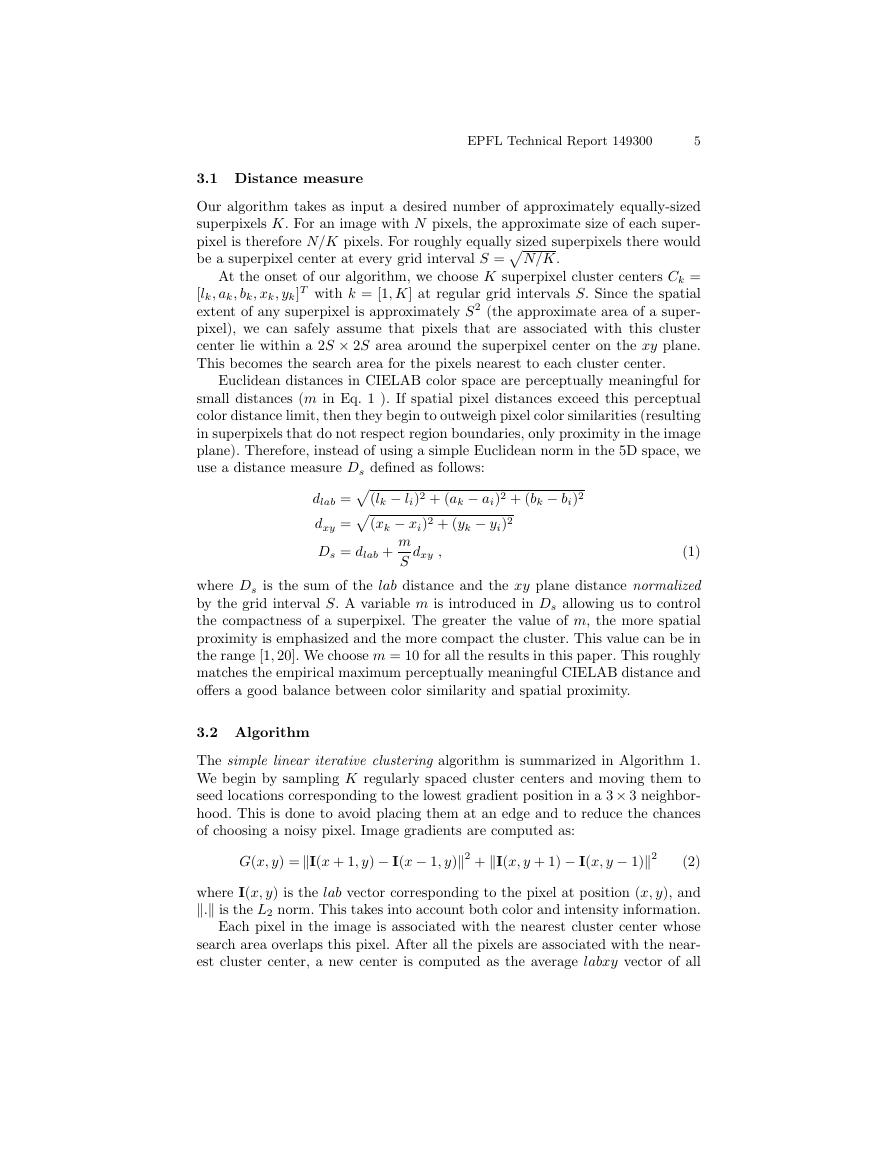
dlab =(lk − li)2 + (ak − ai)2 + (bk − bi)2
dxy =(xk − xi)2 + (yk − yi)2
Ds = dlab + m
S
dxy ,
(1)
where Ds is the sum of the lab distance and the xy plane distance normalized
by the grid interval S. A variable m is introduced in Ds allowing us to control
the compactness of a superpixel. The greater the value of m, the more spatial
proximity is emphasized and the more compact the cluster. This value can be in
the range [1, 20]. We choose m = 10 for all the results in this paper. This roughly
matches the empirical maximum perceptually meaningful CIELAB distance and
offers a good balance between color similarity and spatial proximity.
3.2 Algorithm
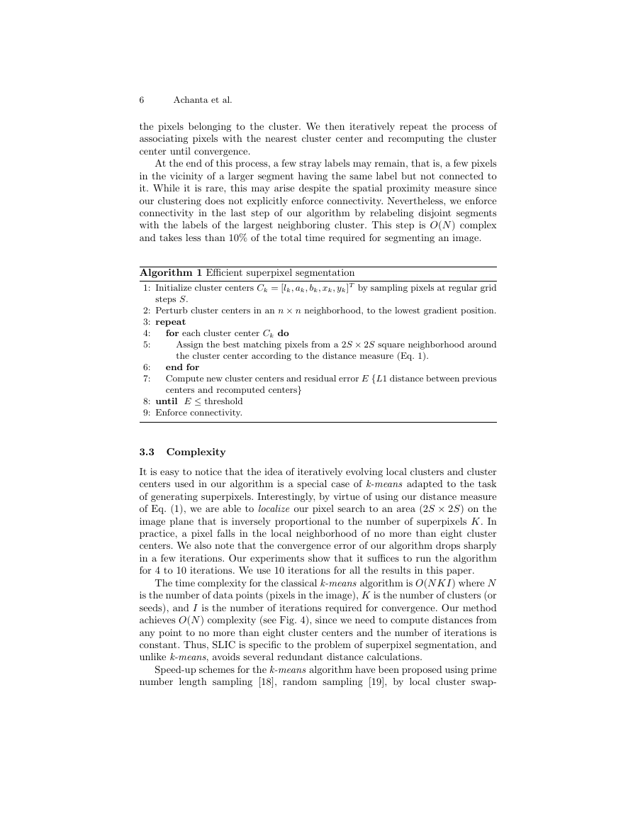
The simple linear iterative clustering algorithm is summarized in Algorithm 1.
We begin by sampling K regularly spaced cluster centers and moving them to
seed locations corresponding to the lowest gradient position in a 3× 3 neighbor-
hood. This is done to avoid placing them at an edge and to reduce the chances
of choosing a noisy pixel. Image gradients are computed as:
G(x, y) =I(x + 1, y) − I(x − 1, y)2 + I(x, y + 1) − I(x, y − 1)2
(2)
where I(x, y) is the lab vector corresponding to the pixel at position (x, y), and
. is the L2 norm. This takes into account both color and intensity information.
Each pixel in the image is associated with the nearest cluster center whose
search area overlaps this pixel. After all the pixels are associated with the near-
est cluster center, a new center is computed as the average labxy vector of all
�
6
Achanta et al.
the pixels belonging to the cluster. We then iteratively repeat the process of
associating pixels with the nearest cluster center and recomputing the cluster
center until convergence.
At the end of this process, a few stray labels may remain, that is, a few pixels
in the vicinity of a larger segment having the same label but not connected to
it. While it is rare, this may arise despite the spatial proximity measure since
our clustering does not explicitly enforce connectivity. Nevertheless, we enforce
connectivity in the last step of our algorithm by relabeling disjoint segments
with the labels of the largest neighboring cluster. This step is O(N) complex
and takes less than 10% of the total time required for segmenting an image.
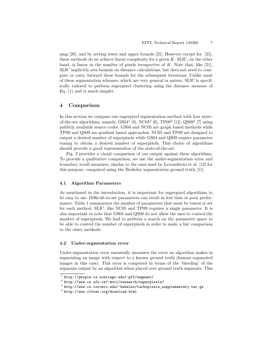
steps S.
Algorithm 1 Efficient superpixel segmentation
1: Initialize cluster centers Ck = [lk, ak, bk, xk, yk]T by sampling pixels at regular grid
2: Perturb cluster centers in an n × n neighborhood, to the lowest gradient position.
3: repeat
4:
5:
Assign the best matching pixels from a 2S × 2S square neighborhood around
the cluster center according to the distance measure (Eq. 1).
for each cluster center Ck do
end for
Compute new cluster centers and residual error E {L1 distance between previous
centers and recomputed centers}
6:
7:
8: until E ≤ threshold
9: Enforce connectivity.
3.3 Complexity
It is easy to notice that the idea of iteratively evolving local clusters and cluster
centers used in our algorithm is a special case of k-means adapted to the task
of generating superpixels. Interestingly, by virtue of using our distance measure
of Eq. (1), we are able to localize our pixel search to an area (2S × 2S) on the
image plane that is inversely proportional to the number of superpixels K. In
practice, a pixel falls in the local neighborhood of no more than eight cluster
centers. We also note that the convergence error of our algorithm drops sharply
in a few iterations. Our experiments show that it suffices to run the algorithm
for 4 to 10 iterations. We use 10 iterations for all the results in this paper.
The time complexity for the classical k-means algorithm is O(N KI) where N
is the number of data points (pixels in the image), K is the number of clusters (or
seeds), and I is the number of iterations required for convergence. Our method
achieves O(N) complexity (see Fig. 4), since we need to compute distances from
any point to no more than eight cluster centers and the number of iterations is
constant. Thus, SLIC is specific to the problem of superpixel segmentation, and
unlike k-means, avoids several redundant distance calculations.
Speed-up schemes for the k-means algorithm have been proposed using prime
number length sampling [18], random sampling [19], by local cluster swap-
�
EPFL Technical Report 149300
7
ping [20], and by setting lower and upper bounds [21]. However except for [21],
these methods do no achieve linear complexity for a given K. SLIC, on the other
hand, is linear in the number of pixels irrespective of K. Note that, like [21],
SLIC implicitly sets bounds on distance calculations, but does not need to com-
pute or carry forward these bounds for the subsequent iterations. Unlike most
of these segmentation schemes, which are very general in nature, SLIC is specif-
ically tailored to perform superpixel clustering using the distance measure of
Eq. (1) and is much simpler.
4 Comparison
In this section we compare our superpixel segmentation method with four state-
of-the-art algorithms, namely, GS041 [8], NC052 [6], TP093 [12], QS094 [7] using
publicly available source codes. GS04 and NC05 are graph based methods while
TP09 and QS09 are gradient based approaches. NC05 and TP09 are designed to
output a desired number of superpixels while GS04 and QS09 require parameter
tuning to obtain a desired number of superpixels. This choice of algorithms
should provide a good representation of the state-of-the-art.
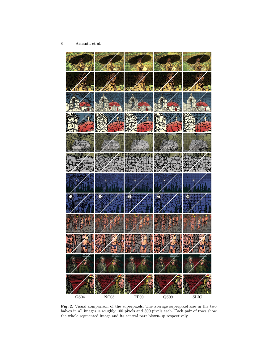
Fig. 2 provides a visual comparison of our output against these algorithms.
To provide a qualitative comparison, we use the under-segmentation error and
boundary recall measures, similar to the ones used by Levenshtein et al. [12] for
this purpose, computed using the Berkeley segmentation ground truth [11].
4.1 Algorithm Parameters
As mentioned in the introduction, it is important for superpixel algorithms to
be easy to use. Difficult-to-set parameters can result in lost time or poor perfor-
mance. Table 1 summarizes the number of parameters that must be tuned or set
for each method. SLIC, like NC05 and TP09 requires a single parameter. It is
also important to note that GS04 and QS09 do not allow the user to control the
number of superpixels. We had to perform a search on the parameter space to
be able to control the number of superpixels in order to make a fair comparison
to the other methods.
4.2 Under-segmentation error
Under-segmentation error essentially measures the error an algorithm makes in
segmenting an image with respect to a known ground truth (human segmented
images in this case). This error is computed in terms of the ‘bleeding’ of the
segments output by an algorithm when placed over ground truth segments. This
1 http://people.cs.uchicago.edu/~pff/segment/
2 http://www.cs.sfu.ca/~mori/research/superpixels/
3 http://www.cs.toronto.edu/~babalex/turbopixels_supplementary.tar.gz
4 http://www.vlfeat.org/download.html
�
8
Achanta et al.
GS04
NC05
TP09
QS09
SLIC
Fig. 2. Visual comparison of the superpixels. The average superpixel size in the two
halves in all images is roughly 100 pixels and 300 pixels each. Each pair of rows show
the whole segmented image and its central part blown-up respectively.
�


 2023年江西萍乡中考道德与法治真题及答案.doc
 2012年重庆南川中考生物真题及答案.doc
 2013年江西师范大学地理学综合及文艺理论基础考研真题.doc
 2020年四川甘孜小升初语文真题及答案I卷.doc
 2020年注册岩土工程师专业基础考试真题及答案.doc
 2023-2024学年福建省厦门市九年级上学期数学月考试题及答案.doc
 2021-2022学年辽宁省沈阳市大东区九年级上学期语文期末试题及答案.doc
 2022-2023学年北京东城区初三第一学期物理期末试卷及答案.doc
 2018上半年江西教师资格初中地理学科知识与教学能力真题及答案.doc
 2012年河北国家公务员申论考试真题及答案-省级.doc
 2020-2021学年江苏省扬州市江都区邵樊片九年级上学期数学第一次质量检测试题及答案.doc
 2022下半年黑龙江教师资格证中学综合素质真题及答案.doc