A Gentle Introduction to Predictive Filters
Siome Klein Goldenstein1
Abstract: Predictive lters are essential tools in modern science. They perform
state prediction and parameter estimation in elds such as robotics, computer vi-
sion, and computer graphics. Sometimes also called Bayesian lters, they apply the
Bayesian rule of conditional probability to combine a predicted behavior with some
corrupted indirect observation.
When we study and solve a problem, we rst need its proper mathematical formula-
tion. Finding the essential parameters that best describe the system is hard, modeling
their behaviors over time is even more challenging. Usually, we also have an in-
spection mechanism, that provides us indirect measurements, the observations, of the
hidden underlying parameters. We also need to deal with the concept of uncertainty,
and use random variables to represent both the state and the observations.
Predictive lters are a family of estimation techniques. They combine the system’s
dynamics uncertain prediction and the corrupted observation. There are many differ-
ent predictive lters, each dealing with different types of mathematical representations
for random variables and system dynamics.
Here, the reader will nd a dense introduction to predictive lters. After a general in-
troduction, we have a brief discussion about mathematical modeling of systems: state
representation, dynamics, and observation. Then, we expose some basic issues related
with random variables and uncertainty modeling, and discuss four implementations
of predictive lters, in order of complexity: the Kalman lter, the extended Kalman
lter, the particle lter, and the unscented Kalman lter.
1
Introduction
In applied sciences, we use mathematical models to describe, understand, and deal
with real objects. Applications are varied, and may involve guiding a mobile exploratory
vehicle, understanding a human face and its expressions, or controlling a nuclear power plant
reactor. A good mathematical representation lets us infer properties of the real entity, and
understand beforehand the possible implications of our interactions with it.
The state vector of a model is the set of parameters that uniquely describe a cong-
uration of the object. The set of parameters that model an object is usually not unique, and
each situation leads to a different set of design choices. When the object’s parameters are not
1Instituto de Computaªo, UNICAMP
Caixa Postal 6176, Campinas - SP, 13084-971 Brazil
siome@ic.unicamp.br
�
A Gentle Introduction to Predictive Filters
static, we also need a mathematical model for their change over time. We call a system, the
mathematical representation of states and dynamics.
Sometimes, the parameters we choose to represent a system are intrinsic to the prob-
lem but impossible to be measured, such as the temperature in the core of a nuclear power
plant. Fortunately, we can usually measure other quantities that are related to the unknown,
but essential parameter, such as the temperature of the cooling water leaving the core. These
indirect measurements are called observations, and can be used to infer information about
the hidden parameter.
Real life is hard, and full of errors. The observations we make are not precise, and they
may not explain all that is happening in the system. Also, our mathematical representation
of the model is not exact, giving slightly incorrect results. To cope with all these factors, we
need to incorporate the notion of uncertainties. There are many mathematical descriptions
for uncertainties, but in this paper we use probabilities.
Predictive lters estimate the optimal state of a system. First, they use the mathemat-
ical model of the system dynamics to propagate the state’s values and uncertainties. Later,
they combine this preliminary estimate and as much as it is possible from the observation.
There are several predictive lters, each appropriate for a different type of uncertainty repre-
sentation and dynamic modeling.
The Kalman lter is the simplest example of a predictive lter. It represents uncertain-
ties as Gaussian random variables, fully described by a mean and a covariance matrix, and
models the system with linear dynamics and observations. Since Gaussians are preserved
under linear transformation, the Kalman lter’s implementation uses only linear algebra op-
erations.
If we need more complex models to describe a system, we may have to use nonlin-
ear functions. The extended Kalman lter linearizes the system around the current state to
propagate and estimate covariance matrices.
We can represent the random variables as a collection of samples, and allow nonlinear
operations. In this case, we can use a particle lter, which is powerful and exible. Unfortu-
nately, it needs an a number of samples exponentially related to the state’s dimension.
Here, the last predictive lter we talk about is the unscented Kalman lter. It uses
a small number of specially selected particles to propagate random variables over nonlinear
transformations.
In this paper, we follow the same type of structure of Maybeck’s classical book [20].
In Section 2, we deal with the problem of building a mathematical model that describes the
state of the system (Section 2.1), its dynamics (Section 2.2), and how to inspect it at every
moment (Section 2.3). Then, in Section 3, we review uncertainties: probabilities and random
2
RITA Volume Nœmero 2004
�
A Gentle Introduction to Predictive Filters
variables. Finally, in Section 4, we describe the Bayesian concepts of predictive lters, and
look at some of its concrete implementations: the Kalman lter (Section 4.1), the extended
Kalman lter (Section 4.2), the particle lter (Section 4.3), and the unscented particle lter
(Section 4.4). In Section 5, we conclude this paper with a series of words of caution, as well
as a series of pointers to where the reader can nd more information.
2 System Representation
Predictive ltering techniques rely on a mathematical representation of the system. In
this section, we discuss how to model a system’s parameters and their dynamical aspects, and
how to describe our indirect ability to inspect them.
A system is just like a black box, controlled by a set of parameters. To manipulate
and understand a system, we need a mathematical model that describes these parameters and
their behavior over time.
There are three general guidelines to modeling: rst, the mathematical model should
be as precise as possible the system’s behavior model should be as close as possible to
reality. Second, the model should be tractable we need to handle the mathematical model
in a efcient way. Finally, the model should be as simple as possible there is no need to
describe a detail of the system, if this detail holds no consequence to the desired application.
Usually, these three guidelines are incompatible, and we have to strike a balance. In the next
three sections we describe the ideas behind state description, the observation procedure, and
the dynamic behavior.
2.1 State Description
We use several real-valued variables to describe a system state.2 If we use n parame-
ters to describe the system, we group them in a vector
~xt 2 Rn;
that uniquely identies the system’s situation at time t. We now look at two examples.
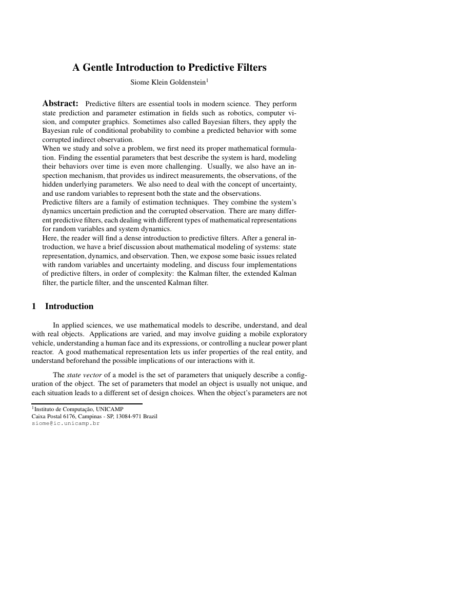
Example 1: Simple Robot Lets consider a mobile robot, that can turn around its axes and
move in the forward direction. We know that the robot cannot leave the oor, so we only
need two coordinates to describe its position. We also need a third parameter to describe its
facing direction. This is illustrated in Figure 1.
2It is possible, and sometimes more adequate, to model systems with graphs and discrete variables, but that is beyond
the scope of this paper.
RITA Volume Nœmero 2004
3
�
A Gentle Introduction to Predictive Filters
PSfrag replacements
y
~x =2
4
x
y
3
5
x
Figure 1. A simple state model of a robot, with x and y positions and forward direction :
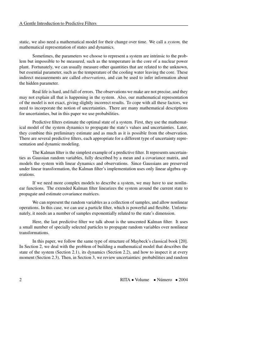
Example 2: Human Face When we look at a human face as a system, we can model de-
formation parameters. These parameters describe the effects of the muscles’ action on the
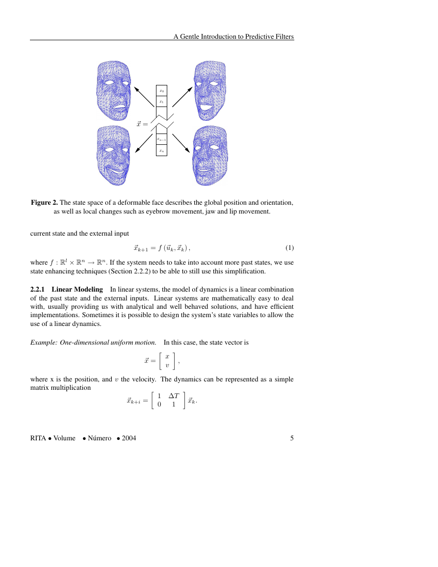
surface of the face. In Figure 2 we see an illustration of how the state vector can affect the
overall shape and position of a face.
2.2 Dynamic Behavior
In order to describe the dynamic behavior of a system, we take into account its state
history and some external inputs, represented as ~uk 2 Rl. In control theory, we use the
mathematical model, along with the initial conguration of the state, to plan the input ~u
over time. This planned ~u guides the system’s state according to our goals. In Bayesian
state estimation, we do not know what the inputs really are (perhaps just some statistics), but
estimate the best state conguration using indirect observations.
There are two models for the passage of time, continuous and discrete. In the rst one,
time is a value t 2 R: In the second representation, time is a integer variable k 2 Z: Usually,
the discrete time approach is considered an uniform sampling t = k T of the continuous
case. In this paper, we will only use the discrete representation.
A natural representation for the dynamics of discrete-time system is a difference equa-
tion. The next state depends on the current input and all the system’s history
~xk+1 = f (~uk; ~xk; : : : ; ~x0) :
Fortunately, it is usually enough to consider that the next state depends only on the
4
RITA Volume Nœmero 2004
�
A Gentle Introduction to Predictive Filters
PSfrag replacements
x0
x1
xn1
xn
~x =
Figure 2. The state space of a deformable face describes the global position and orientation,
as well as local changes such as eyebrow movement, jaw and lip movement.
current state and the external input
(1)
where f : Rl Rn ! Rn: If the system needs to take into account more past states, we use
state enhancing techniques (Section 2.2.2) to be able to still use this simplication.
~xk+1 = f (~uk; ~xk) ;
2.2.1 Linear Modeling In linear systems, the model of dynamics is a linear combination
of the past state and the external inputs. Linear systems are mathematically easy to deal
with, usually providing us with analytical and well behaved solutions, and have efcient
implementations. Sometimes it is possible to design the system’s state variables to allow the
use of a linear dynamics.
Example: One-dimensional uniform motion.
In this case, the state vector is
~x = x
v ;
where x is the position, and v the velocity. The dynamics can be represented as a simple
matrix multiplication
~xk+i = 1 T
1 ~xk:
0
RITA Volume Nœmero 2004
5
�
A Gentle Introduction to Predictive Filters
In general, the system depends on m different inputs ~uk 2 Rm; and we represent the
system dynamics through the difference equation
~xk+1 = A~xk + B~uk;
where A 2 Rnn; and B 2 Rnm:
2.2.2 State Enhancing Techniques During the mathematical modeling stage, there are
many tricks we can play with the description and representation of a system. For example,
suppose we need a more powerful model of dynamics than of Equation 1, one that takes into
account the two previous states,
In order to use the one-state history formulation for systems, all need a change of variables
~xk+1 = g (~uk; ~xk; ~xk1) :
~Xk+1 = ~xk
~xk1 ;
where ~Xi 2 R2m: The dynamics can then be written as
~Xk+1 = f~uk; ~Xk =" g~uk; In
0n ~Xk; 0n
0n ~Xk
In
In ~Xk
# ;
where In is the n-dimension identity matrix, and 0n is the n-dimension zero valued matrix. It
is worth noting that this technique is not limited to linear dynamics, and can take into account
any nite number of previous states. In calculus, this idea is used to rewrite a high-degree
differential equation as a system of rst-degree differential equations.
2.3 Observation
To complete our mathematical formulation, we need to model the observation. An
observation ~y 2 Rm is an indirect measurement of the state’s value
~yk = h (~xk; ~uk) :
(2)
In Section 4, we will see how to combine the information from the prediction from the system
dynamics (Equation 1) and the observation, to obtain the best possible estimation.
3 Uncertainty Modeling
In prediction, estimation, and control, we have to deal with inexact quantities. There
are different options to model and represent uncertainties, such as intervals and regions of
6
RITA Volume Nœmero 2004
�
A Gentle Introduction to Predictive Filters
condence [23, 24, 40], or random variables and probabilities [6, 27, 42]. In this paper, we
only use of random variables.
In this section, we briey describe a few common terms and expressions from prob-
ability theory. For a short and good introduction, look for Chapter 2 in Wozencraft’s classic
communication book [42].
Probability System A probability system is a mathematical model composed by three enti-
ties: a sample space, a set of events, and a probability measure dened on these events. The
sample space (generally referred to by the symbol ) is a collection of possibilities, objects.
An object in is called a sample point, and is denoted !: An event is a set of sample points,
and a probability measure is the assignment of real numbers to the events dened on ; such
that this assignment satises the following conditions:
1. To every event Ai; there is a unique number P [Ai] assigned such that 0 P [Ai] 1:
2. P [] = 1:
3. If two events A and B are disjoint, AT B = ; P [AS B] = P [A] + P [B] :
Conditional Probability The knowledge about an event give us information regarding other
events as well. If we know that an experiment of the sample space belongs to event B; then
the probability of it being also part of event A is no longer P [A] : Effectively, in this case
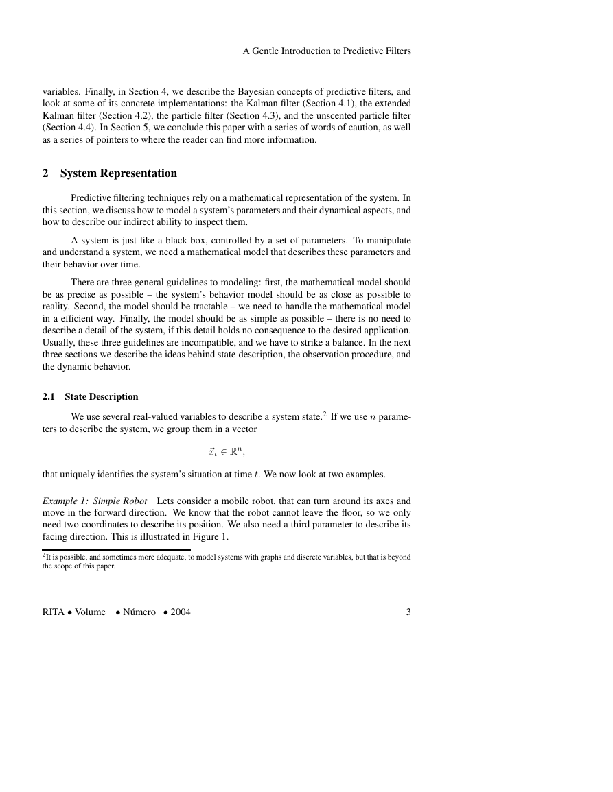
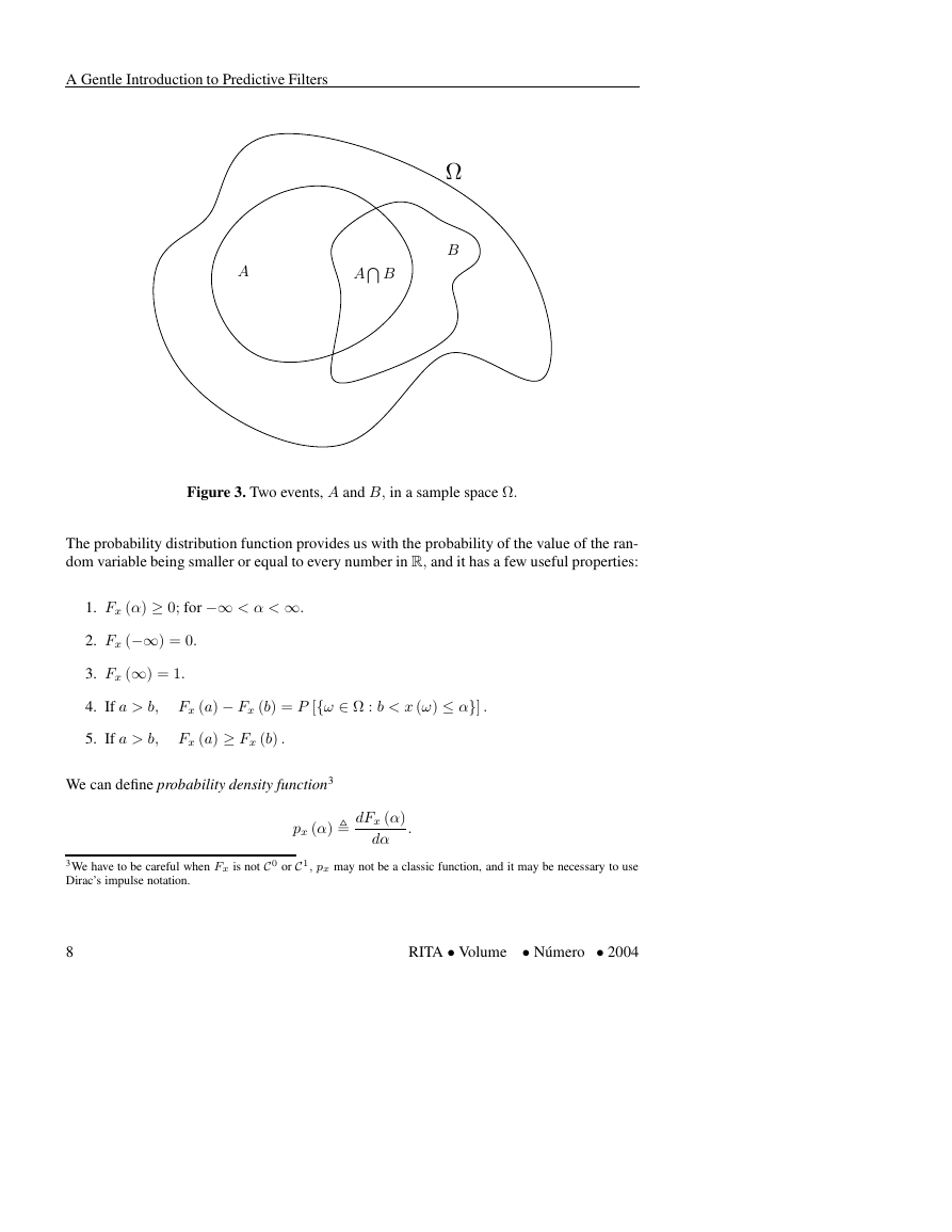
we narrow our sample space to the subspace B of : In Figure 3 we can see a Venn diagram
representing ; A; and B:
If we know that an experiment lies in B; and that P [B] 6= 0; then the probability that
this experiment also lie on A is the conditional probability
P [A \ B]
:
P [AjB] ,
P [B]
(3)
When P [A] is also nonzero, we can write
P [A \ B] = P [AjB] P [B] = P [BjA] P [A] :
This conditional probability relation is called Bayes rule, and it is the essence of the
predictive, or Bayesian, lters.
Random Variables A random variable is a mapping x (!) : ! R of all samples from
to R: We call the probability distribution function
Fx () , P [f! 2 : x (!) g] :
RITA Volume Nœmero 2004
(4)
7
�
A Gentle Introduction to Predictive Filters
B
A
AT B
PSfrag replacements
Figure 3. Two events, A and B; in a sample space :
The probability distribution function provides us with the probability of the value of the ran-
dom variable being smaller or equal to every number in R; and it has a few useful properties:
1. Fx () 0; for 1 < < 1:
2. Fx (1) = 0:
3. Fx (1) = 1:
4. If a > b; Fx (a) Fx (b) = P [f! 2 : b < x (!) g] :
5. If a > b; Fx (a) Fx (b) :
We can dene probability density function3
px () ,
dFx ()
d
:
3We have to be careful when Fx is not C 0 or C 1; px may not be a classic function, and it may be necessary to use
Dirac’s impulse notation.
8
RITA Volume Nœmero 2004
�


 2023年江西萍乡中考道德与法治真题及答案.doc
 2012年重庆南川中考生物真题及答案.doc
 2013年江西师范大学地理学综合及文艺理论基础考研真题.doc
 2020年四川甘孜小升初语文真题及答案I卷.doc
 2020年注册岩土工程师专业基础考试真题及答案.doc
 2023-2024学年福建省厦门市九年级上学期数学月考试题及答案.doc
 2021-2022学年辽宁省沈阳市大东区九年级上学期语文期末试题及答案.doc
 2022-2023学年北京东城区初三第一学期物理期末试卷及答案.doc
 2018上半年江西教师资格初中地理学科知识与教学能力真题及答案.doc
 2012年河北国家公务员申论考试真题及答案-省级.doc
 2020-2021学年江苏省扬州市江都区邵樊片九年级上学期数学第一次质量检测试题及答案.doc
 2022下半年黑龙江教师资格证中学综合素质真题及答案.doc