GPS Tool Box The GPS Easy Suite–Matlab code for the GPS newcomer Kai Borre Abstract The Matlab computing environment has become a popular way to perform complex matrix calculations, and to produce sophisticated graphics output in a relatively easy manner. Large collections of Matlab scripts are now available for a wide variety of applications and are often used for university courses. The GPS Easy Suite is a collection of ten Matlab scripts, or M-files, which can be used by those just beginning to learn about GPS. The first few scripts perform basic GPS calculations such as converting GPS Time in year/month/day/hour/ minute/second format to GPS week/seconds of week, computing the position of a satellite using a broadcast ephemeris, and computing the coordinates of a single point using pseudorange observations. The latter scripts can perform calculations such as computing baseline components using either traditional least-squares or a Kalman filter, fixing cycle slips and millisecond clock jumps, and computing ionospheric delay using carrier phase observations. I describe the purpose of each M-file and give graphical results based on real data. The Matlab code and the sample datasets are available from my website. I have also included additional text files (in pdf format) to discuss the various Time Systems and Coordinate Systems used in GPS computations, and to show the equations used for computing the position of a satellite using the ephemeris information broadcast from the satellites. Received: 8 January 2003 / Accepted: 24 January 2003 Published online: 4 April 2003 ª Springer-Verlag 2003 K. Borre Danish GPS Center, Aalborg University, Niels Jernes Vej 14, 9220 Aalborg, Denmark E-mail: borre@gps.auc.dk Tel.: +45-9635-8362 Fax: +45-9815-1583 Introduction I seldom teach the same course the same way. Often I start afresh. Last autumn I tried a new approach to lecturing my Introductory GPS Computations class. Courses in my de- partment run in modules of six lectures; so I split up the basic issues into six lectures containing the following topics: – time: Universal Time, GPS Time (GPS week and seconds of week), Modified Julian Date, Leap Seconds, Interna- tional Atomic Time, Terrestrial Dynamical Time (see time_itr.pdf on the web at http://www.gps.auc.dk/ ~borre/easy; – Kepler’s laws, computation of satellite position (see Strang and Borre 1997, pages 482–487); – observation types, computation of receiver position (see Strang and Borre 1997, pages 463–465, 460–461); – observational errors, differencing techniques, Dilution of Precision (DOP) (see Strang and Borre 1997, pages 453–460, 462–463, 465–467); – computation of a baseline from pseudoranges; – computation of a baseline from pseudoranges and phase observations (see Strang and Borre 1997, page 463). Some reflections resulted in four additional topics: – estimation of the receiver clock offset (see Strang and Borre 1997, pages 507–509); – cycle-slip detection and repair of millisecond receiver clock resets (see Strang and Borre 1997, pages 491, 509); – various representations of an estimated baseline (see Strang and Borre 1997, pages 367–368, 472–475, 501–502); – ionospheric delay estimated from carrier phase observations F1 and F2 (see Strang and Borre 1997, page 490). The basic GPS datasets we will be working with were collected at Aalborg by two JPS Eurocard receivers on 4 September 2001. The resulting Receiver Independent Exchange (RINEX) files (Gurtner 2000) are site247j.01o, site24~1.01o, and site247j.01n. For the more specialized topics we need a longer observation series; this is contained in file kofi1.01o. We number the Matlab scripts easy1 to easy10; hence, they more or less relate to the ten topics listed above. All files are zipped and are available via the world wide web at http://www.gps.auc.dk/~borre/easy. DOI 10.1007/s10291-003-0049-3 GPS Solutions (2003) 7:47–51 47 

GPS Tool Box Much of the theoretical background for the easy scripts can be found in chapters 14 and 15 of Strang and Borre (1997). However, we wanted to add some additional text here to emphasize certain issues which are central to the code but often are not mentioned in textbooks. Below follows a description of the various M-scripts. The Easy Suite easy1 Nearly any GPS processing starts with time issues. Easy1 shows how to convert a given epoch, originating from one of the RINEX Observation files (O-files), to GPS week and seconds of week (sow). We include the time_itr.pdf file which is a text file which gives an overview of relevant timescales and reference frames useful for GPS. easy2 The second basic computation is to calculate the position in the Earth-Centered, Earth-Fixed frame (ECEF) of a given PRN at a given time. For a given time and an ephemeris obtained from a RINEX Navigation Message file (N-file), easy2 does the job. The main function is satpos which is an implementation of the procedure described in the GPS Interface Control Document (ICD-GPS-200C 1997), Table 20-IV. We read a RINEX N-file and reformat it into Matlab’s internal format, namely, a matrix named Eph. Furthermore, we relate each PRN to a column of Eph. Each column contains 21 variables; these comprise a complete ephemeris for one satellite. easy3 In easy3 we compute a receiver’s ECEF position from RINEX O- and N-files. Only pseudoranges are used. The computation is repeated over 20 epochs. Each position is the result of an iterative least-squares procedure. 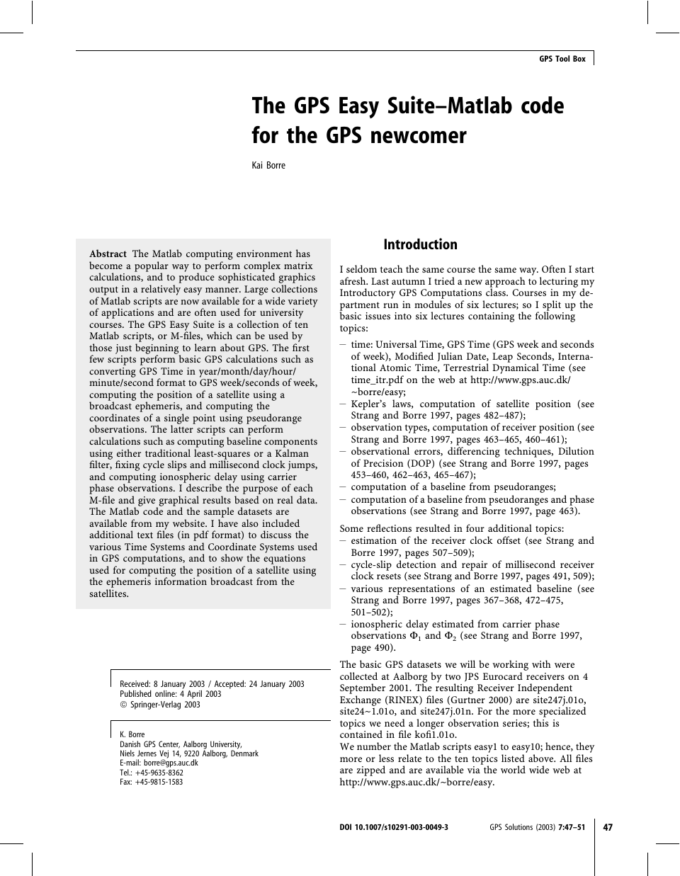The variation of the position relative to the first epoch is shown in Fig. 1. The variation in coordinate values is typically less than 5 m. We open a RINEX O-file and read all the pseudoranges given at an epoch. With given satellite positions from easy2, we compute the receiver position. Fig. 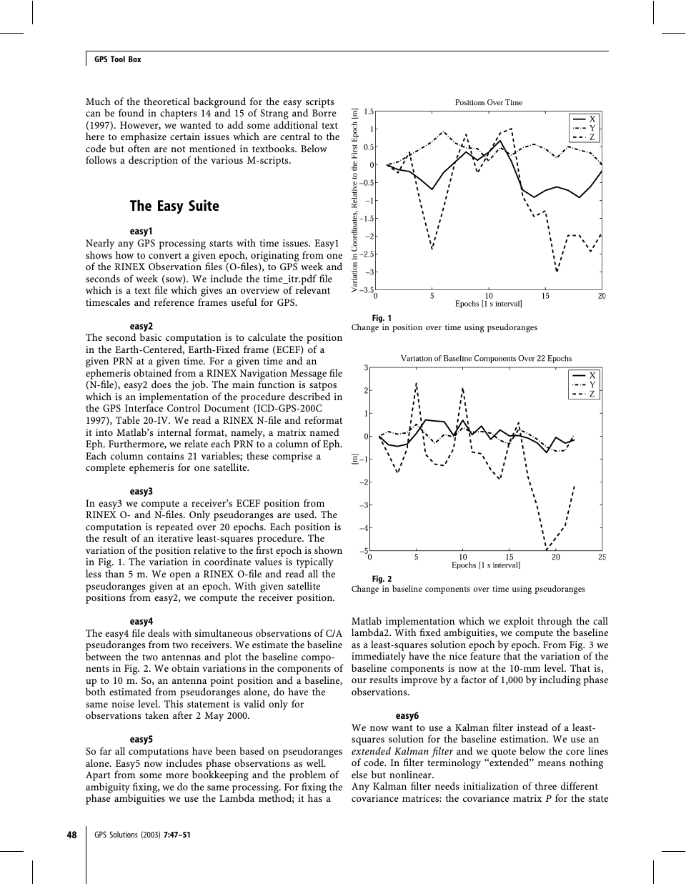1 Change in position over time using pseudoranges Fig. 2 Change in baseline components over time using pseudoranges easy4 The easy4 file deals with simultaneous observations of C/A pseudoranges from two receivers. We estimate the baseline between the two antennas and plot the baseline compo- nents in Fig. 2. We obtain variations in the components of up to 10 m. So, an antenna point position and a baseline, both estimated from pseudoranges alone, do have the same noise level. This statement is valid only for observations taken after 2 May 2000. easy5 So far all computations have been based on pseudoranges alone. Easy5 now includes phase observations as well. Apart from some more bookkeeping and the problem of ambiguity fixing, we do the same processing. For fixing the phase ambiguities we use the Lambda method; it has a Matlab implementation which we exploit through the call lambda2. 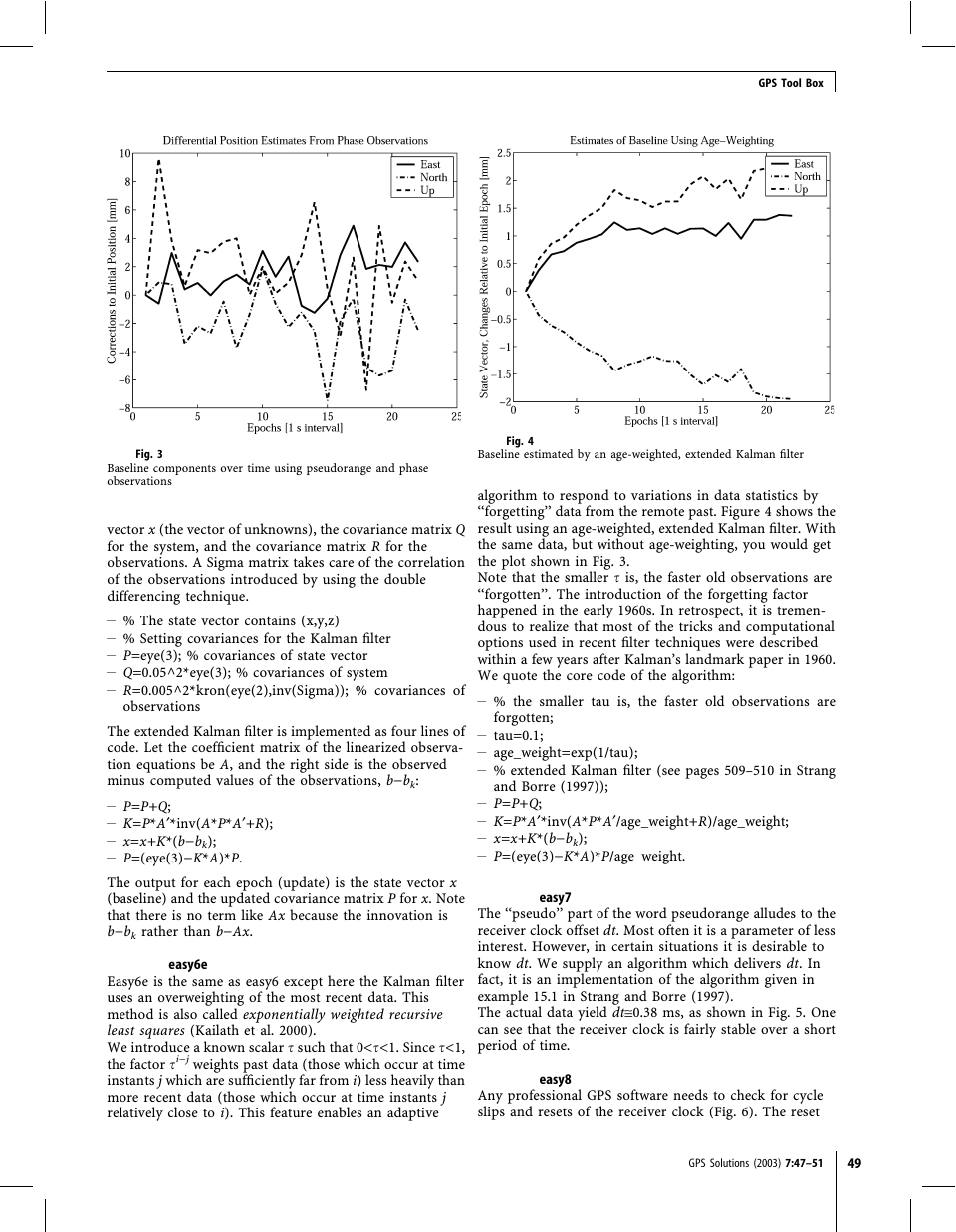With fixed ambiguities, we compute the baseline as a least-squares solution epoch by epoch. From Fig. 3 we immediately have the nice feature that the variation of the baseline components is now at the 10-mm level. That is, our results improve by a factor of 1,000 by including phase observations. easy6 We now want to use a Kalman filter instead of a least- squares solution for the baseline estimation. We use an extended Kalman filter and we quote below the core lines of code. In filter terminology ‘‘extended’’ means nothing else but nonlinear. Any Kalman filter needs initialization of three different covariance matrices: the covariance matrix P for the state 48 GPS Solutions (2003) 7:47–51 

GPS Tool Box Fig. 3 Baseline components over time using pseudorange and phase observations vector x (the vector of unknowns), the covariance matrix Q for the system, and the covariance matrix R for the observations. A Sigma matrix takes care of the correlation of the observations introduced by using the double differencing technique. – % The state vector contains (x,y,z) – % Setting covariances for the Kalman filter – P=eye(3); % covariances of state vector – Q=0.05^2*eye(3); % covariances of system – R=0.005^2*kron(eye(2),inv(Sigma)); % covariances of observations The extended Kalman filter is implemented as four lines of code. Let the coefficient matrix of the linearized observa- tion equations be A, and the right side is the observed minus computed values of the observations, b)bk: – P=P+Q; – K=P*A¢*inv(A*P*A¢+R); – x=x+K*(b)bk); – P=(eye(3))K*A)*P. The output for each epoch (update) is the state vector x (baseline) and the updated covariance matrix P for x. Note that there is no term like Ax because the innovation is b)bk rather than b)Ax. easy6e Easy6e is the same as easy6 except here the Kalman filter uses an overweighting of the most recent data. This method is also called exponentially weighted recursive least squares (Kailath et al. 2000). 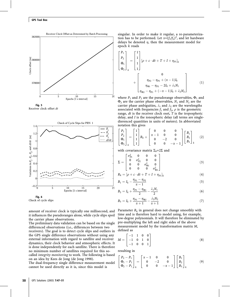We introduce a known scalar s such that 0

GPS Tool Box Fig. 5 Receiver clock offset dt Fig. 6 Check of cycle slips amount of receiver clock is typically one millisecond, and it influences the pseudoranges alone, while cycle slips spoil the carrier phase observations. The preliminary data validation can be based on the single differenced observations (i.e., differences between two receivers). The goal is to detect cycle slips and outliers in the GPS single difference observations without using any external information with regard to satellite and receiver dynamics, their clock behavior and atmospheric effects. It is done independently for each satellite. There is therefore no minimum number of satellites required for this so- called integrity monitoring to work. The following is based on an idea by Kees de Jong (de Jong 1998). The dual-frequency single difference measurement model cannot be used directly as it is, since this model is 50 GPS Solutions (2003) 7:47–51 singular. In order to make it regular, a re-parameteriza- tion has to be performed. Let a=(f1/f2)2, and let hardware delays be denoted g, then the measurement model for 3 2 2 epoch k reads 6664 6664 7775 q þ c
dt þ T þ I þ gP1 3 7775 ¼ 1 1 ½ Šk P1 P2 U1 U2 1 2 1 6664 k þ 3 7775 ð1Þ 0 ÞIk gP2 gP1 þ a 1 gU1 gP1 2Ik þ k1N1 ð gU2 gP1 þ a 1 ð ÞIk þ k2N2 where P1 and P2 are the pseudorange observables, F1 and F2 are the carrier phase observables, N1 and N2 are the carrier phase ambiguities, k1 and k2 are the wavelengths associated with frequencies f1 and f2, q is the geometric range, dt is the receiver clock oset, T is the tropospheric delay, and I is the ionospheric delay (all terms are single- dierenced quantities in units of meters). In abbreviated 2 notation this gives 664 3 2 775 B1 4 3 775 2 664 3 775 2 664 3 5 ¼ Rk þ ð2Þ 0 a 1 0 0 0 0 0 0 0 2 0 a 1 P1 P2 U1 U2 1 1 1 1 B2 B3 with covariance matrix Sb=2S and k 2 664 r2 P1 0 0 0 R ¼ 3 775 0 r2 P2 0 0 0 0 r2 U1 0 0 0 0 r2 U2 Šk ½ Rk ¼ q þ c
dt þ T þ I þ gP1 B1 ¼ Ik gP1 gP2 a 1 B2 ¼ Ik þ gP1 gU1 B3 ¼ Ik þ gP1 gU2 a þ 1 k1N1 2 k2N2 a þ 1 2 k ð3Þ ð4Þ ð5Þ ð6Þ ð7Þ 3 5 2 4 Parameter Rk in general does not change smoothly with time and is therefore hard to model using, for example, low-degree polynomials. It will therefore be eliminated by pre-multiplying the left and right sides of the above measurement model by the transformation matrix M, defined as 1 1 1 3 2 resulting in P2 P1 4 5 U1 P1 U2 P1 0 2 0 a 1 2 3 4 5 B1 B2 B3 a 1 0 0 0 1 0 2 4 M ¼ 3 5 ð9Þ ð8Þ 1 0 0 0 0 1 ¼ 0 0 k k 

GPS Tool Box with covariance matrix M Sb MT. The parameters B1, B2, and B3 are linear combinations of the time-dependent ionospheric eect and the constant hardware delays and carrier ambiguities. The ionospheric eect will be modeled as a first-order polynomial, i.e., as a bias Ik and a drift _IIk.     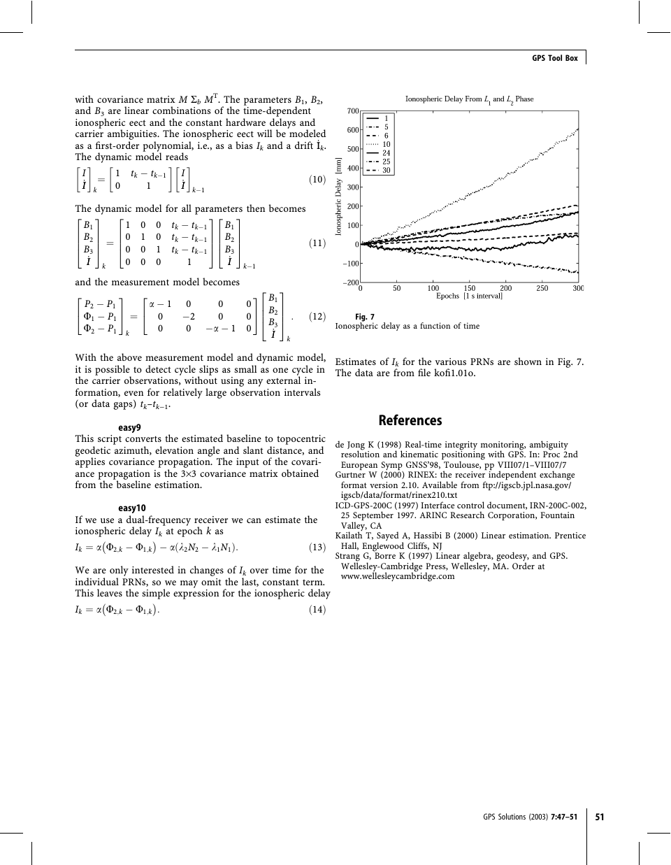The dynamic model reads I I _II _II tk tk1 ð10Þ  1 k1 2 The dynamic model for all parameters then becomes 664 3 2 775 B1 664 3 775 3 775 ð11Þ tk tk1 tk tk1 tk tk1 1 0 0 1 0 B2 B3 _II k  ¼ 1 0 2 664 ¼ k B1 B2 B3 _II 1 0 0 0 3 5 0 1 0 0 2 4 2 and the measurement model becomes 4 P2 P1 U1 P1 U2 P1 ¼ k a 1 0 0 0 0 0 2 0 a 1 k1 2 3 664 5 B1 B2 B3 _II 0 0 0 3 775 k ð12Þ : Fig. 7 Ionospheric delay as a function of time With the above measurement model and dynamic model, it is possible to detect cycle slips as small as one cycle in the carrier observations, without using any external in- formation, even for relatively large observation intervals (or data gaps) tk–tk)1. easy9 This script converts the estimated baseline to topocentric geodetic azimuth, elevation angle and slant distance, and applies covariance propagation. The input of the covari- ance propagation is the 3·3 covariance matrix obtained from the baseline estimation. easy10 If we use a dual-frequency receiver we can estimate the ionospheric delay Ik at epoch k as Ik ¼ a U2;k U1;k a k2N2 k1N1 Þ:
ð ð13Þ We are only interested in changes of Ik over time for the individual PRNs, so we may omit the last, constant term. This leaves the simple expression for the ionospheric delay Ik ¼ a U2;k U1;k ð14Þ
: Estimates of Ik for the various PRNs are shown in Fig. 7. The data are from file kofi1.01o. References de Jong K (1998) Real-time integrity monitoring, ambiguity resolution and kinematic positioning with GPS. In: Proc 2nd European Symp GNSS’98, Toulouse, pp VIII07/1–VIII07/7 Gurtner W (2000) RINEX: the receiver independent exchange format version 2.10. Available from ftp://igscb.jpl.nasa.gov/ igscb/data/format/rinex210.txt ICD-GPS-200C (1997) Interface control document, IRN-200C-002, 25 September 1997. ARINC Research Corporation, Fountain Valley, CA Kailath T, Sayed A, Hassibi B (2000) Linear estimation. Prentice Hall, Englewood Cliffs, NJ Strang G, Borre K (1997) Linear algebra, geodesy, and GPS. Wellesley-Cambridge Press, Wellesley, MA. Order at www.wellesleycambridge.com GPS Solutions (2003) 7:47–51 51