Durrett的概率论.pdf-资料库

qq_33598125-10811230-16359647436848504894.pdf-第1页.png

第1页 / 共122页

qq_33598125-10811230-16359647436848504894.pdf-第2页.png

第2页 / 共122页

qq_33598125-10811230-16359647436848504894.pdf-第3页.png

第3页 / 共122页

qq_33598125-10811230-16359647436848504894.pdf-第4页.png

第4页 / 共122页

qq_33598125-10811230-16359647436848504894.pdf-第5页.png

第5页 / 共122页

qq_33598125-10811230-16359647436848504894.pdf-第6页.png

第6页 / 共122页

qq_33598125-10811230-16359647436848504894.pdf-第7页.png

第7页 / 共122页

qq_33598125-10811230-16359647436848504894.pdf-第8页.png

第8页 / 共122页

Probability: Theory and Examples Solutions Manual The creation of this solution manual was one of the most important im- provements in the second edition of Probability: Theory and Examples. The solutions are not intended to be as polished as the proofs in the book, but are supposed to give enough of the details so that little is left to the reader’s imag- ination. It is inevitable that some of the many solutions will contain errors. If you ﬁnd mistakes or better solutions send them via e-mail to rtd1@cornell.edu or via post to Rick Durrett, Dept. of Math., 523 Malott Hall, Cornell U., Ithaca NY 14853. Rick Durrett

Contents 1 Laws of Large Numbers 1 3 7 1 1. Basic Deﬁnitions 2. Random Variables 3. Expected Value 4 4. Independence 5. Weak Laws of Large Numbers 6. Borel-Cantelli Lemmas 7. Strong Law of Large Numbers 8. Convergence of Random Series 9. Large Deviations 15 24 12 19 20 2 Central Limit Theorems 26 1. The De Moivre-Laplace Theorem 26 27 2. Weak Convergence 3. Characteristic Functions 4. Central Limit Theorems 6. Poisson Convergence 39 7. Stable Laws 8. Inﬁnitely Divisible Distributions 9. Limit theorems in Rd 31 35 43 45 46 3 Random walks 48 1. Stopping Times 48 4. Renewal theory 51

4 Martingales 54 Contents iii 43 1. Conditional Expectation 54 2. Martingales, Almost Sure Convergence 3. Examples 4. Doob’s Inequality, Lp Convergence 5. Uniform Integrability, Convergence in L1 6. Backwards Martingales 68 7. Optional Stopping Theorems 64 69 57 66 5 Markov Chains 74 74 1. Deﬁnitions and Examples 2. Extensions of the Markov Property 75 3. Recurrence and Transience 4. Stationary Measures 5. Asymptotic Behavior 6. General State Space 82 84 88 79 6 Ergodic Theorems 91 91 1. Deﬁnitions and Examples 2. Birkhoﬀ’s Ergodic Theorem 93 3. Recurrence 6. A Subadditive Ergodic Theorem 96 7. Applications 95 97 7 Brownian Motion 98 1. Deﬁnition and Construction 98 2. Markov Property, Blumenthal’s 0-1 Law 99 3. Stopping Times, Strong Markov Property 100 4. Maxima and Zeros 5. Martingales 102 6. Donsker’s Theorem 105 7. CLT’s for Dependent Variables 8. Empirical Distributions, Brownian Bridge 9. Laws of the Iterated Logarithm 107 101 106 107

iv Contents Appendix: Measure Theory 108 108 1. Lebesgue-Stieltjes Measures 2. Carath´eodary’s Extension Theorem 109 3. Completion, etc. 4. Integration 109 5. Properties of the Integral 6. Product Measures, Fubini’s Theorem 114 8. Radon-Nikodym Theorem 116 109 112

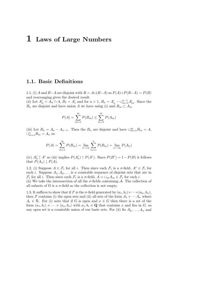
1 Laws of Large Numbers 1.1. Basic Deﬁnitions 1.1. (i) A and B−A are disjoint with B = A∪(B−A) so P (A)+P (B−A) = P (B) and rearranging gives the desired result. (ii) Let A0 m=1A0 Bn are disjoint and have union A we have using (i) and Bm ⊂ Am n = An ∩ A, B1 = A0 n − ∪n−1 m. Since the 1 and for n > 1, Bn = A0 ∞X P (Bm) ≤ ∞X P (Am) m=1 m=1 P (A) = (iii) Let Bn = An − An−1. Then the Bn are disjoint and have ∪∞ ∪n m=1Bm = An so m=1Bm = A, ∞X m=1 nX m=1 P (A) = P (Bm) = lim n→∞ P (Bm) = lim n→∞ P (An) n ↑ Ac so (iii) implies P (Ac n) ↑ P (Ac). Since P (Bc) = 1− P (B) it follows (iv) Ac that P (An) ↓ P (A). 1.2. (i) Suppose A ∈ Fi for all i. Then since each Fi is a σ-ﬁeld, Ac ∈ Fi for each i. Suppose A1, A2, . . . is a countable sequence of disjoint sets that are in Fi for all i. Then since each Fi is a σ-ﬁeld, A = ∪mAm ∈ Fi for each i. (ii) We take the interesection of all the σ-ﬁelds containing A. The collection of all subsets of Ω is a σ-ﬁeld so the collection is not empty. 1.3. It suﬃces to show that if F is the σ-ﬁeld generated by (a1, b1)×···×(an, bn), then F contains (i) the open sets and (ii) all sets of the form A1 ×··· An where Ai ∈ R. For (i) note that if G is open and x ∈ G then there is a set of the form (a1, b1) × ··· × (an, bn) with ai, bi ∈ Q that contains x and lies in G, so any open set is a countable union of our basic sets. For (ii) ﬁx A2, . . . , An and

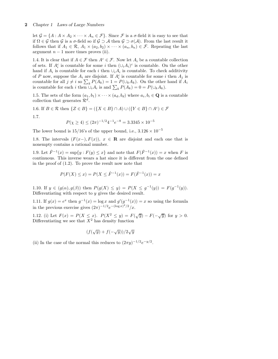
2 Chapter 1 Laws of Large Numbers let G = {A : A × A2 × ··· × An ∈ F}. Since F is a σ-ﬁeld it is easy to see that if Ω ∈ G then G is a σ-ﬁeld so if G ⊃ A then G ⊃ σ(A). From the last result it follows that if A1 ∈ R, A1 × (a2, b2) × ··· × (an, bn) ∈ F. Repeating the last argument n − 1 more times proves (ii). 1.4. It is clear that if A ∈ F then Ac ∈ F. Now let Ai be a countable collection i is countable for some i then (∪iAi)c is countable. On the other of sets. If Ac hand if Ai is countable for each i then ∪iAi is countable. To check additivity countable for all j 6= i soPk P (Ak) = 1 = P (∪kAk). On the other hand if Ai of P now, suppose the Ai are disjoint. If Ac i is countable for some i then Aj is is countable for each i then ∪iAi is andPk P (Ak) = 0 = P (∪kAk). 1.5. The sets of the form (a1, b1) × ··· × (ad, bd) where ai, bi ∈ Q is a countable collection that generates Rd. 1.6. If B ∈ R then {Z ∈ B} = ({X ∈ B} ∩ A) ∪ ({Y ∈ B} ∩ Ac) ∈ F 1.7. P (χ ≥ 4) ≤ (2π)−1/24−1e −8 = 3.3345 × 10−5 The lower bound is 15/16’s of the upper bound, i.e., 3.126 × 10−5 1.8. The intervals (F (x−), F (x)), x ∈ R are disjoint and each one that is nonempty contains a rational number. 1.9. Let ˆF −1(x) = sup{y : F (y) ≤ x} and note that F ( ˆF −1(x)) = x when F is continuous. This inverse wears a hat since it is diﬀerent from the one deﬁned in the proof of (1.2). To prove the result now note that −1(x)) = F ( ˆF P (F (X) ≤ x) = P (X ≤ ˆF −1(x)) = x 1.10. If y ∈ (g(α), g(β)) then P (g(X) ≤ y) = P (X ≤ g−1(y)) = F (g−1(y)). Diﬀerentiating with respect to y gives the desired result. 1.11. If g(x) = ex then g−1(x) = log x and g0(g−1(x)) = x so using the formula in the previous exercise gives (2π)−1/2e−(log x)2/2/x. √ 1.12. (i) Let F (x) = P (X ≤ x). P (X 2 ≤ y) = F ( Diﬀerentiating we see that X 2 has density function √ y))/2 y) − F (−√ y) + f(−√ y) for y > 0. √ (f( y (ii) In the case of the normal this reduces to (2πy)−1/2e−y/2.

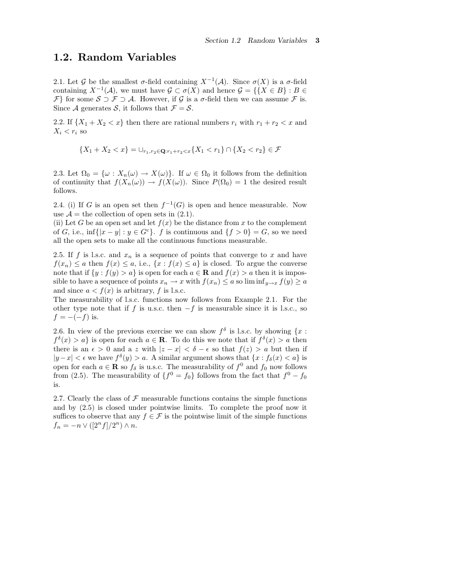
Section 1.2 Random Variables 3 1.2. Random Variables 2.1. Let G be the smallest σ-ﬁeld containing X−1(A). Since σ(X) is a σ-ﬁeld containing X−1(A), we must have G ⊂ σ(X) and hence G = {{X ∈ B} : B ∈ F} for some S ⊃ F ⊃ A. However, if G is a σ-ﬁeld then we can assume F is. Since A generates S, it follows that F = S. 2.2. If {X1 + X2 < x} then there are rational numbers ri with r1 + r2 < x and Xi < ri so {X1 + X2 < x} = ∪r1,r2∈Q:r1+r2 0} = G, so we need all the open sets to make all the continuous functions measurable. 2.5. If f is l.s.c. and xn is a sequence of points that converge to x and have f(xn) ≤ a then f(x) ≤ a, i.e., {x : f(x) ≤ a} is closed. To argue the converse note that if {y : f(y) > a} is open for each a ∈ R and f(x) > a then it is impos- sible to have a sequence of points xn → x with f(xn) ≤ a so lim inf y→x f(y) ≥ a and since a < f(x) is arbitrary, f is l.s.c. The measurability of l.s.c. functions now follows from Example 2.1. For the other type note that if f is u.s.c. then −f is measurable since it is l.s.c., so f = −(−f) is. 2.6. In view of the previous exercise we can show f δ is l.s.c. by showing {x : f δ(x) > a} is open for each a ∈ R. To do this we note that if f δ(x) > a then there is an > 0 and a z with |z − x| < δ − so that f(z) > a but then if |y− x| < we have f δ(y) > a. A similar argument shows that {x : fδ(x) < a} is open for each a ∈ R so fδ is u.s.c. The measurability of f 0 and f0 now follows from (2.5). The measurability of {f 0 = f0} follows from the fact that f 0 − f0 is. 2.7. Clearly the class of F measurable functions contains the simple functions and by (2.5) is closed under pointwise limits. To complete the proof now it suﬃces to observe that any f ∈ F is the pointwise limit of the simple functions fn = −n ∨ ([2nf]/2n) ∧ n.

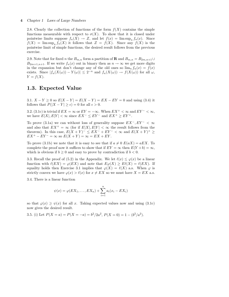
4 Chapter 1 Laws of Large Numbers 2.8. Clearly the collection of functions of the form f(X) contains the simple functions measurable with respect to σ(X). To show that it is closed under pointwise limits suppose fn(X) → Z, and let f(x) = lim supn fn(x). Since f(X) = lim supn fn(X) it follows that Z = f(X). Since any f(X) is the pointwise limit of simple functions, the desired result follows from the previous exercise. 2.9. Note that for ﬁxed n the Bm,n form a partition of R and Bm,n = B2m,n+1∪ B2m+1,n+1. If we write fn(x) out in binary then as n → ∞ we get more digits in the expansion but don’t change any of the old ones so limn fn(x) = f(x) exists. Since |fn(X(ω)) − Y (ω)| ≤ 2−n and fn(X(ω)) → f(X(ω)) for all ω, Y = f(X). 1.3. Expected Value 3.1. X − Y ≥ 0 so E|X − Y | = E(X − Y ) = EX − EY = 0 and using (3.4) it follows that P (|X − Y | ≥ ) = 0 for all > 0. 3.2. (3.1c) is trivial if EX = ∞ or EY = −∞. When EX + < ∞ and EY − < ∞, we have E|X|, E|Y | < ∞ since EX− ≤ EY − and EX + ≥ EY +. To prove (3.1a) we can without loss of generality suppose EX−, EY − < ∞ and also that EX + = ∞ (for if E|X|, E|Y | < ∞ the result follows from the theorem). In this case, E(X + Y )− ≤ EX− + EY − < ∞ and E(X + Y )+ ≥ EX + − EY − = ∞ so E(X + Y ) = ∞ = EX + EY . To prove (3.1b) we note that it is easy to see that if a 6= 0 E(aX) = aEX. To complete the proof now it suﬃces to show that if EY = ∞ then E(Y + b) = ∞, which is obvious if b ≥ 0 and easy to prove by contradiction if b < 0. 3.3. Recall the proof of (5.2) in the Appendix. We let `(x) ≤ ϕ(x) be a linear function with `(EX) = ϕ(EX) and note that Eϕ(X) ≥ E`(X) = `(EX). If equality holds then Exercise 3.1 implies that ϕ(X) = `(X) a.s. When ϕ is strictly convex we have ϕ(x) > `(x) for x 6= EX so we must have X = EX a.s. 3.4. There is a linear function ψ(x) = ϕ(EX1, . . . , EXn) + ai(xi − EXi) nX so that ϕ(x) ≥ ψ(x) for all x. Taking expected values now and using (3.1c) now gives the desired result. 3.5. (i) Let P (X = a) = P (X = −a) = b2/2a2, P (X = 0) = 1 − (b2/a2). i=1

资料库

Durrett的概率论.pdf

相关推荐

课程资源

热门标签

最新资料