566
IEEE TRANSACTIONS ON CONTROL SYSTEMS TECHNOLOGY, VOL. 15, NO. 3, MAY 2007
Predictive Active Steering Control for Autonomous
Vehicle Systems
Paolo Falcone, Francesco Borrelli, Jahan Asgari, Hongtei Eric Tseng, and Davor Hrovat, Fellow, IEEE
Abstract—In this paper, a model predictive control (MPC)
approach for controlling an active front steering system in an
autonomous vehicle is presented. At each time step, a trajectory is
assumed to be known over a finite horizon, and an MPC controller
computes the front steering angle in order to follow the trajectory
on slippery roads at the highest possible entry speed. We present
two approaches with different computational complexities. In
the first approach, we formulate the MPC problem by using a
nonlinear vehicle model. The second approach is based on suc-
cessive online linearization of the vehicle model. Discussions on
computational complexity and performance of the two schemes
are presented. The effectiveness of the proposed MPC formulation
is demonstrated by simulation and experimental tests up to 21 m/s
on icy roads.
Index Terms—Active steering, autonomous vehicles, model pre-
dictive control, nonlinear optimization, vehicle dynamics control,
vehicle stability.
I. INTRODUCTION
R ECENT trends in automotive industry point in the di-
rection of increased content of electronics, computers,
and controls with emphasis on the improved functionality
and overall system robustness. While this affects all of the
vehicle areas, there is a particular interest in active safety,
which effectively complements the passive safety counterpart.
Passive safety is primarily focused on the structural integrity
of vehicle. Active safety on the other hand is primarily used to
avoid accidents and at the same time facilitate better vehicle
controllability and stability especially in emergency situations,
such as what may occur when suddenly encountering slippery
parts of the road [10].
Early works on active safety systems date back to the 1980s
and were primarily focused on improving longitudinal dy-
namics part of motion, in particular, on more effective braking
(ABS) and traction control (TC) systems. ABS systems in-
crease the braking efficiency by avoiding the lock of the braking
wheels. TC systems prevent the wheel from slipping and at the
same time improves vehicle stability and steerability by maxi-
mizing the tractive and lateral forces between the vehicle’s tire
and the road. This was followed by work on different vehicle
Manuscript received November 10, 2006. Manuscript received in final form
January 12, 2007. Recommended by Associate Editor K. Fishbach.
P. Falcone and F. Borrelli are with the Universitá del Sannio, Dipartimento di
Ingegneria, Università degli Studi del Sannio, 82100 Benevento, Italy (e-mail:
falcone@unisannio.it; francesco.borrelli@unisannio.it).
J. Asgari, H. E. Tseng, and D. Hrovat are with Research and Innovation
Center, Ford Research Laboratories, Dearborn, MI 48124 USA (e-mail: jas-
gari@ford.com; htseng@ford.com; dhrovat@ford.com).
Color versions of Figs. 1, 2, and 4–12 are available online at http://ieeexplore.
ieee.org.
Digital Object Identifier 10.1109/TCST.2007.894653
stability control systems [34] (which are also known under
different acronyms such as electronic stability program (ESP),
vehicle stability control (VSC), interactive vehicle dynamics
(IVD), and dynamic stability control (DSC)). Essentially, these
systems use brakes on one side and engine torque to stabilize
the vehicle in extreme limit handling situations through con-
trolling the yaw motion.
In addition to braking and traction systems, active front
steering (AFS) systems make use of the front steering com-
mand in order to improve lateral vehicle stability [1], [2].
Moreover, the steering command can be used to reject ex-
ternal destabilizing forces arising from -split, asymmetric
braking, or wind [21]. Four-wheel steer (4WS) systems follow
similar goals. For instance, in [3], Ackermann et al. present a
decoupling strategy between the path following and external
disturbances rejection in a four-wheel steering setup. The
automatic car steering is split into the path following and the
yaw stabilization tasks, the first is achieved through the front
steering angle, the latter through the rear steering angle.
Research on the AFS systems has also been approached
from an autonomous vehicle perspective. In [16], an automatic
steering control for highway automation is presented, where
the vehicle is equipped with magnetic sensors placed on the
front and rear bumpers in order to detect a lane reference im-
plemented with electric wire [13] and magnetic markers [36].
A more recent example of AFS applications in autonomous
vehicles is the “Grand Challenge” race driving [5], [23], [30].
In this paper, it is anticipated that the future systems will be
able to increase the effectiveness of active safety interventions
beyond what is currently available. This will be facilitated not
only by additional actuator types such as 4WS, active steering,
active suspensions, or active differentials, but also by additional
sensor information, such as onboard cameras, as well as in-
frared and other sensor alternatives. All these will be further
complemented by global positioning system (GPS) information
including prestored mapping. In this context, it is possible to
imagine that future vehicles would be able to identify obstacles
on the road such as an animal, a rock, or fallen tree/branch, and
assist the driver by following the best possible path, in terms of
avoiding the obstacle and at the same time keeping the vehicle on
the road at a safe distance from incoming traffic. An additional
source of information can also come from surrounding vehicles
and environments which may convey the information from the
vehicle ahead about road condition, which can give a significant
amount of preview to the controller. This is particular is useful
if one travels on snow or ice covered surfaces. In this case, it is
very easy to reach the limit of vehicle handling capabilities.
Anticipating sensor and infrastructure trends toward in-
creased integration of information and control actuation agents,
1063-6536/$25.00 © 2007 IEEE
�
FALCONE et al.: PREDICTIVE ACTIVE STEERING CONTROL FOR AUTONOMOUS VEHICLE SYSTEMS
567
it is then appropriate to ask what is the optimum way in con-
trolling the vehicle maneuver for a given obstacle avoidance
situation.
We assume that a trajectory planning system is available and
we consider a double lane change scenario on a slippery road,
with a vehicle equipped with a fully autonomous guidance
system. In this paper, we focus on the control of the yaw and
lateral vehicle dynamics via active front steering. The control
input is the front steering angle and the goal is to follow the
desired trajectory or target as close as possible while fulfilling
various constraints reflecting vehicle physical limits and design
requirements. The future desired trajectory is known only over
finite horizon at each time step. This is done in the spirit of
model predictive control (MPC) [14], [26] along the lines of
our ongoing internal research efforts dating from early 2000
(see [7] and references therein).
In this paper, two different formulations of the AFS MPC
problem will be presented and compared. The first one follows
the work presented in [7] and uses a nonlinear vehicle model
to predict the future evolution of the system [26]. The resulting
MPC controller requires a nonlinear optimization problem to
be solved at each time step. We will show that the computa-
tional burden is currently an obstacle for experimental valida-
tion at high vehicle speed. The second formulation tries to over-
come this problem and presents a suboptimal MPC controller
based on successive online linearization of the nonlinear vehicle
model. This is linearized around the current operating point at
each time step and a linear MPC controller is designed for the re-
sulting linear time-varying (LTV) system. The idea of using time
varying models goes back to the early 1970s in the process con-
trol field although it has been properly formalized only recently.
Studies on linear parameter varying (LPV) MPC schemes can be
found in [9], [18], [20], [22], and [35]. Among them, the work
in [18] and [20] is the closest to our approach and it presents
an MPC scheme for scheduled LTV models which has been
successfully validated on a Boeing aircraft. In general, the per-
formance of such a scheme is highly dependant on the nonlin-
earities of the model. In fact, as the state and input trajectories
deviate from the current operating point, the model mismatch
increases. This can generate large prediction errors with a con-
sequent instability of the closed-loop system. We will show that,
in our application, a state constraint can be introduced in order
to significantly enhance the performance of the system. Exper-
imental results show that the vehicle can be stabilized up to
21 m/s on icy roads. Finally, an LTV MPC with a one-step con-
trol horizon is presented. This can be tuned in order to provide
acceptable performance and it does not require any complex op-
timization software.
We implemented the MPC controllers in real time on a pas-
senger car, and performed tests on snow covered and icy roads.
The last part of this paper describes the experimental setup and
presents the experimental and simulation results of the proposed
MPC controllers. It should be noted that our early work in [7]
focuses on the vehicle dynamical model and on simulation re-
sults of the nonlinear MPC scheme only.
This paper is structured as follows. Section II describes
the used vehicle dynamical model with a brief discussion on
tire models. Section III introduces a simplified hierarchical
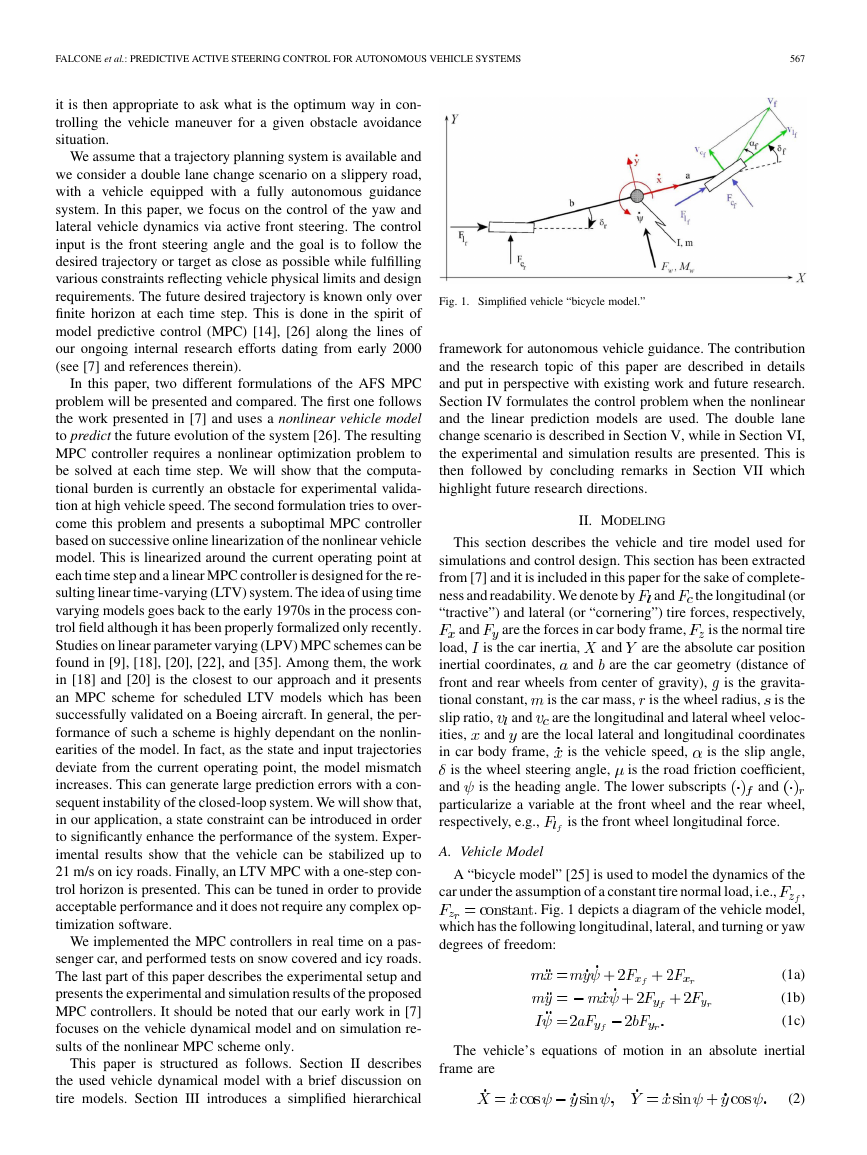
Fig. 1. Simplified vehicle “bicycle model.”
framework for autonomous vehicle guidance. The contribution
and the research topic of this paper are described in details
and put in perspective with existing work and future research.
Section IV formulates the control problem when the nonlinear
and the linear prediction models are used. The double lane
change scenario is described in Section V, while in Section VI,
the experimental and simulation results are presented. This is
then followed by concluding remarks in Section VII which
highlight future research directions.
II. MODELING
and
are the forces in car body frame,
This section describes the vehicle and tire model used for
simulations and control design. This section has been extracted
from [7] and it is included in this paper for the sake of complete-
the longitudinal (or
ness and readability. We denote by
“tractive”) and lateral (or “cornering”) tire forces, respectively,
is the normal tire
and
are the absolute car position
are the car geometry (distance of
is the gravita-
is the
is the car mass,
are the longitudinal and lateral wheel veloc-
are the local lateral and longitudinal coordinates
is the slip angle,
is the road friction coefficient,
load,
inertial coordinates,
front and rear wheels from center of gravity),
tional constant,
and
slip ratio,
ities,
in car body frame,
is the wheel steering angle,
is the vehicle speed,
is the wheel radius,
and
is the car inertia,
and
and
is the heading angle. The lower subscripts
and
particularize a variable at the front wheel and the rear wheel,
respectively, e.g.,
is the front wheel longitudinal force.
and
A. Vehicle Model
car under the assumption of a constant tire normal load, i.e.,
A “bicycle model” [25] is used to model the dynamics of the
,
. Fig. 1 depicts a diagram of the vehicle model,
which has the following longitudinal, lateral, and turning or yaw
degrees of freedom:
(1a)
(1b)
(1c)
The vehicle’s equations of motion in an absolute inertial
frame are
(2)
�
568
IEEE TRANSACTIONS ON CONTROL SYSTEMS TECHNOLOGY, VOL. 15, NO. 3, MAY 2007
The wheel’s equations of motion describe the lateral (or cor-
nering) and longitudinal wheel velocities
(3a)
(3b)
(3c)
(3d)
where
tively, and
and
are front and rear wheel steering angle, respec-
(4a)
(4b)
The following equations hold for rear and front axes by using
the corresponding subscript for all the variables. Longitudinal
and lateral tire forces lead to the following forces acting on the
center of gravity:
Tire forces
and
for each tire are given by
(5a)
(6)
,
,
, and
are defined next. The tire slip angle
where
and
represents the angle between the wheel velocity vector
the direction of the wheel itself, and can be compactly expressed
as
The slip ratio
is defined as
if
if
for braking
for driving
(7)
(8)
and
where
are the radius and the angular speed of the wheel,
represents the road friction coef-
respectively. The parameter
ficient and is assumed equal for front and rear wheels.
is the
total vertical load of the vehicle and is distributed between the
front and rear wheels based on the geometry of the car model
(described by the parameters
and )
(9)
The nonlinear vehicle dynamics described in (1)–(9), can be
rewritten in the following compact from:
(10)
and friction coefficient
at each time instant has been explicitly highlighted. The
,
is assumed to be zero at any time
where the dependence on slip ratio
value
state and input vectors are
respectively. In this paper,
instant.
and
Model (10) captures the most relevant nonlinearities associ-
ated to lateral stabilization of the vehicle. Section II-B briefly
describes the models of tire forces
and
.
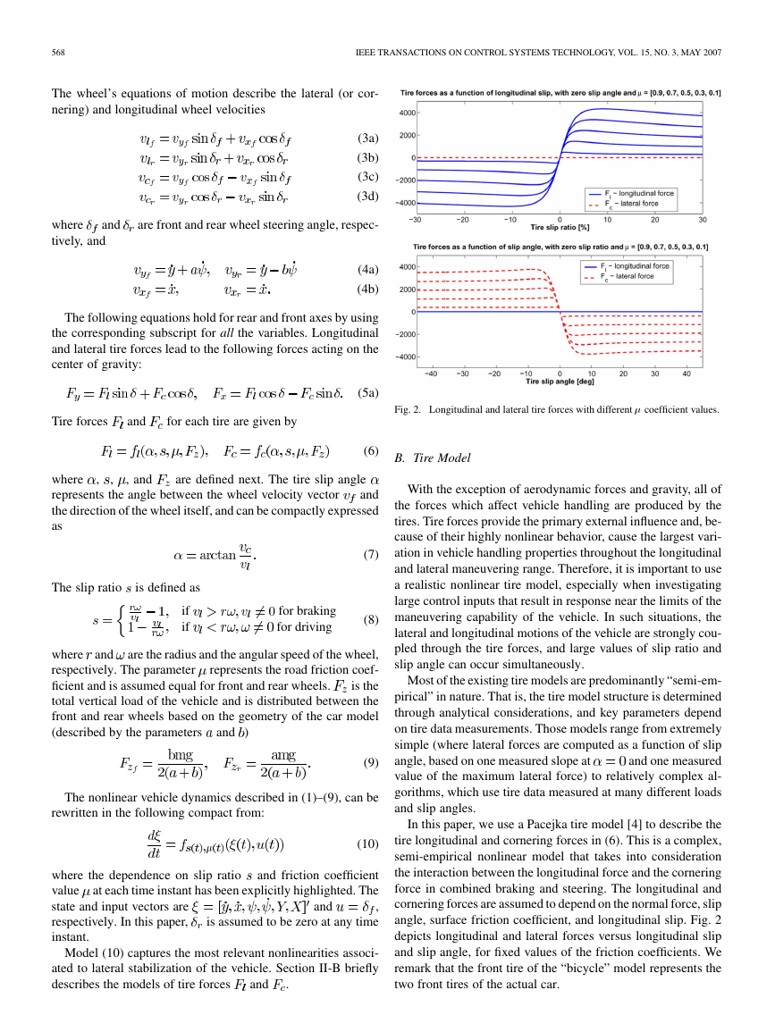
Fig. 2. Longitudinal and lateral tire forces with different � coefficient values.
B. Tire Model
With the exception of aerodynamic forces and gravity, all of
the forces which affect vehicle handling are produced by the
tires. Tire forces provide the primary external influence and, be-
cause of their highly nonlinear behavior, cause the largest vari-
ation in vehicle handling properties throughout the longitudinal
and lateral maneuvering range. Therefore, it is important to use
a realistic nonlinear tire model, especially when investigating
large control inputs that result in response near the limits of the
maneuvering capability of the vehicle. In such situations, the
lateral and longitudinal motions of the vehicle are strongly cou-
pled through the tire forces, and large values of slip ratio and
slip angle can occur simultaneously.
Most of the existing tire models are predominantly “semi-em-
pirical” in nature. That is, the tire model structure is determined
through analytical considerations, and key parameters depend
on tire data measurements. Those models range from extremely
simple (where lateral forces are computed as a function of slip
and one measured
angle, based on one measured slope at
value of the maximum lateral force) to relatively complex al-
gorithms, which use tire data measured at many different loads
and slip angles.
In this paper, we use a Pacejka tire model [4] to describe the
tire longitudinal and cornering forces in (6). This is a complex,
semi-empirical nonlinear model that takes into consideration
the interaction between the longitudinal force and the cornering
force in combined braking and steering. The longitudinal and
cornering forces are assumed to depend on the normal force, slip
angle, surface friction coefficient, and longitudinal slip. Fig. 2
depicts longitudinal and lateral forces versus longitudinal slip
and slip angle, for fixed values of the friction coefficients. We
remark that the front tire of the “bicycle” model represents the
two front tires of the actual car.
�
FALCONE et al.: PREDICTIVE ACTIVE STEERING CONTROL FOR AUTONOMOUS VEHICLE SYSTEMS
569
We remark that the scheme in Fig. 3 is an oversimplified
scheme and that additional hierarchical levels could be present
both in the trajectory/mode replanning module and in the
low-level control system module. The union of the first three
modules is often referred to as guidance and navigation control
(GNC) system.
Typically, the trajectory replanner and the low-level control
system modules do not share the same information on envi-
ronment and vehicle. For instance, the replanning algorithms
can use information coming from cameras or radars which may
not be used at the lower level. Also, typically, the frequency at
which the trajectory replanning module is executed is lower than
the one of the lower level control system. The design of both
modules makes use of vehicle and environment models with
different levels of detail. The fidelity of the dynamical model
used for the design of the two modules is dictated, among many
factors, by a performance/computational resource compromise
and, in the literature, there is no accepted standard on this. One
of the possible control paradigms for the two modules con-
sists in using a high-fidelity vehicle model for designing the
lower level controller while the trajectory planner relies on a
rougher/less detailed dynamical model of the vehicle. Clearly,
the higher the fidelity of the models used at the higher level is,
the easier the job for the lower level control algorithm becomes.
Studies on GNC algorithms vary in 1) the focus (trajectory
replanner and/or the low-level control system); 2) the type of
vehicle dynamical model used; 3) the type of control design
used; and 4) inputs and sensors choice.
In [23], the trajectory replanner module is based on a receding
horizon control design. The planning problem is formulated as a
constrained optimization problem minimizing a weighted sum
of arrival time, steering, and acceleration control efforts. The
vehicle model is a simple rear-centered kinematic model with
acceleration, speed, steering, steering rate, and rollover con-
straints. The lower level control module uses two separated pro-
portional–integral–differentials (PIDs) to control longitudinal
and lateral dynamics. The longitudinal controller acts on throttle
and brakes while the lateral controls on the steering angle.
The GNC architecture in [30] is similar to [23]. The trajectory
planning task is posed as a constrained optimization problem.
The cost function penalizes obstacles collision, distance from
the precomputed offline trajectory and the lateral offset from
the current trajectory. At the lower level, a PI controller acts
on brakes and throttle to control the longitudinal dynamics. A
simple nonlinear controller, instead, is used to control the lateral
dynamics through the steering angle. Details on the vehicle dy-
namical model used in [30] are not disclosed. In [29], a scheme
similar to the one in [23] is used to design a GNC systems for a
flight control application.
In [33], an explicit MPC scheme has been applied at the lower
level control to allocate four wheel slips in order to get a desired
yaw moment. The steering angle is not controlled.
In this paper, we assume that the path can be generated with
two different methods. In the first, the trajectory is established
by simply driving a test vehicle slowly along the desired path,
e.g., a double lane change manoeuvre. The actual path is
recorded by differential GPS and then used as a desired path
for subsequent tests at higher speed. This method has been used
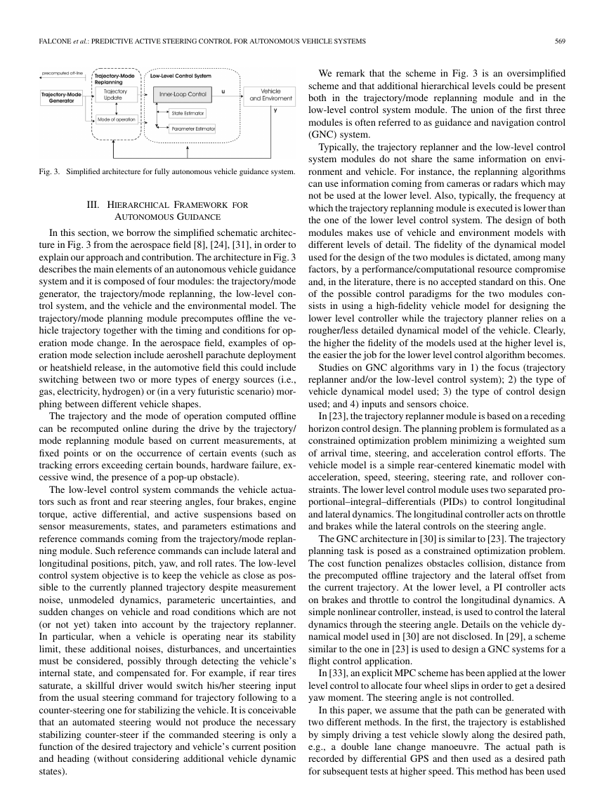
Fig. 3. Simplified architecture for fully autonomous vehicle guidance system.
III. HIERARCHICAL FRAMEWORK FOR
AUTONOMOUS GUIDANCE
In this section, we borrow the simplified schematic architec-
ture in Fig. 3 from the aerospace field [8], [24], [31], in order to
explain our approach and contribution. The architecture in Fig. 3
describes the main elements of an autonomous vehicle guidance
system and it is composed of four modules: the trajectory/mode
generator, the trajectory/mode replanning, the low-level con-
trol system, and the vehicle and the environmental model. The
trajectory/mode planning module precomputes offline the ve-
hicle trajectory together with the timing and conditions for op-
eration mode change. In the aerospace field, examples of op-
eration mode selection include aeroshell parachute deployment
or heatshield release, in the automotive field this could include
switching between two or more types of energy sources (i.e.,
gas, electricity, hydrogen) or (in a very futuristic scenario) mor-
phing between different vehicle shapes.
The trajectory and the mode of operation computed offline
can be recomputed online during the drive by the trajectory/
mode replanning module based on current measurements, at
fixed points or on the occurrence of certain events (such as
tracking errors exceeding certain bounds, hardware failure, ex-
cessive wind, the presence of a pop-up obstacle).
The low-level control system commands the vehicle actua-
tors such as front and rear steering angles, four brakes, engine
torque, active differential, and active suspensions based on
sensor measurements, states, and parameters estimations and
reference commands coming from the trajectory/mode replan-
ning module. Such reference commands can include lateral and
longitudinal positions, pitch, yaw, and roll rates. The low-level
control system objective is to keep the vehicle as close as pos-
sible to the currently planned trajectory despite measurement
noise, unmodeled dynamics, parameteric uncertainties, and
sudden changes on vehicle and road conditions which are not
(or not yet) taken into account by the trajectory replanner.
In particular, when a vehicle is operating near its stability
limit, these additional noises, disturbances, and uncertainties
must be considered, possibly through detecting the vehicle’s
internal state, and compensated for. For example, if rear tires
saturate, a skillful driver would switch his/her steering input
from the usual steering command for trajectory following to a
counter-steering one for stabilizing the vehicle. It is conceivable
that an automated steering would not produce the necessary
stabilizing counter-steer if the commanded steering is only a
function of the desired trajectory and vehicle’s current position
and heading (without considering additional vehicle dynamic
states).
�
570
IEEE TRANSACTIONS ON CONTROL SYSTEMS TECHNOLOGY, VOL. 15, NO. 3, MAY 2007
in [34] to generate the reference path for a steering robot on
high . In this case, no trajectory replanning is needed and the
contribution of the work presented in this paper is to facilitate
systematic and repeatable tests of safety critical emergency
manoeuvres during limit conditions, such as obstacle avoidance
manoeuvres on slippery surfaces, i.e., snow and ice. In the
second method, we assume that a trajectory replanning module
is available and the trajectory is recomputed at a less frequent
rate than the frequency of the lower level controller. For both
cases, we focus on the lower level control design by means of
nonlinear and LTV MPC for the specific scenario of an active
steering system.
As suggested in [28], there is a significant challenge involved
in obtaining the steering required to accomplish the limit ma-
neuver considered in this paper while maintaining vehicle sta-
bility. By focusing on the lower level MPC controller, we also
believe that the resultant steering may mimic a skillful driver
who takes the full vehicle dynamic states into account. Com-
pared to the lower level control algorithms presented in the
aforementioned literature, our approach 1) is model based and
uses the vehicle model (10) and the highly nonlinear Pacejka tire
model described in Section II-B; 2) includes constraints on in-
puts and states in the control design; 3) is systematic and multi-
variable and can accommodate new actuators and higher fidelity
models. Moreover, we have experimentally validated the con-
troller presented in this paper with a dSPACE AutoBox system
which is a standard rapid prototyping system used in automo-
tive industries [11].
nonlinear vehicle model (10) and the Pacejka tire model are
used to predict the future evolution of the system. The mini-
mization of a quadratic performance index, subject to the non-
linear vehicle dynamics, is a nonlinear optimization problem.
Such optimization problem is solved online, at each time step.
This can be computationally demanding, depending on the ve-
hicles states and constraints. The second formulation, presented
in Section IV-B, tries to overcome this problem. A LTV approx-
imation of vehicle model (10) and the Pacejka tire model are
used to predict the future evolution of the system. This leads to
a suboptimal LTV MPC controller. In this case, a time varying
convex quadratic optimization problem is formulated and solved
at each time step, leading to the reduction of the computational
burden with an acceptable loss of performance. We will show
that the MPC performance is enhanced by including a constraint
on the tire slip angle which stabilizes the vehicle at high speed.
A. Nonlinear (NL) MPC
In order to obtain a finite-dimensional optimal control
problem, we discretize the system dynamics (10) with a fixed
sampling time
where the
formulation is used, with
.
(11a)
(11b)
and
IV. ACTIVE STEERING CONTROLLER DESIGN
position states:
In this section, we introduce the control design procedure
for the proposed path following problem via an active steering
system.
(12)
We define the following output map for yaw angle and lateral
, the yaw rate
Desired references for the heading angle
,
define a desired path over a finite
and the lateral distance
horizon. The nonlinear vehicle dynamics (10) and the Pacejka
tire model are used to predict the vehicles behavior, and the front
is chosen as control input. The rear steering
steering angle
and
angle is assumed to be zero
is estimated at each
time instant. The approach used in [6] can be used for the online
estimation of
are measured, and the road friction
, the tire slip ratios
.
and consider the following cost function:
(13)
where
denote the corresponding reference
signal. At each time step , the following finite horizon optimal
control problem is solved:
and
subj. to
A MPC scheme is used to solve the path following problem.
The main concept of MPC is to use a model of the plant to pre-
dict the future evolution of the system [6], [14], [17], [26], [27].
At each sampling time, starting at the current state of the ve-
hicle, an open-loop optimal control problem is solved over a fi-
nite horizon. The open-loop optimal control problem minimizes
the deviations of the predicted outputs from their references over
a sequence of future steering angles, subject to operating con-
straints. The resulting optimal command signal is applied to the
process only during the following sampling interval. At the next
time step, a new optimal control problem based on new mea-
surements of the state is solved over a shifted horizon.
In the following two different formulations of the AFS MPC
problem will be presented. Section IV-A describes the first MPC
formulation as presented in the preliminary work [7]. There, the
(14a)
(14b)
(14c)
(14d)
(14e)
(14f)
(14g)
(14h)
(14i)
�
FALCONE et al.: PREDICTIVE ACTIVE STEERING CONTROL FOR AUTONOMOUS VEHICLE SYSTEMS
571
is the optimization
where
denotes the output vector predicted
vector at time ,
,
at time
and applying to system (11) and (12) the input sequence
denote the output prediction
obtained by starting from the state
and
.
horizon and the control horizon, respectively. We use
and the control signal is assumed constant for all
.
We assume slip and friction coefficient values constant and
over the prediction
equal to the estimated values at time
horizon [constraint (14d)].
In (13), the first summand reflects the penalty on trajectory
tracking error while the second summand is a measure of the
are weighting matrices of appropriate
steering effort.
dimensions.
and
We denote by
the se-
by
. Then, the first
is used to compute the optimal control action
quence of optimal input increments computed at time
solving (14) for the current observed states
sample of
and the resulting state feedback control law is
(15)
, the optimization problem (14) is
At the next time step
solved over a shifted horizon based on the new measurements
of the state
.
B. LTV MPC
Let be the current time and
be the current
state and the previous input of system (11) and (12), respec-
tively. We consider the following optimization problem:
and
subj. to
(16a)
(16b)
(16c)
(16d)
(16e)
(16f)
(16g)
(16h)
(16i)
(16j)
(16k)
(16l)
(16m)
,
around the point
, for the estimated
and
and model (16b) and
where
(16c) is obtained by linearizing model (11) at each time step
.
The variables
denote the outputs
of the linearized system and the corresponding reference signal,
denotes the tire slip angle varia-
respectively. The variable
tion and it is an additional output of the linearized model which
is only constrained and not tracked. Inequalities (16j) are soft
is a slack variable. The
constraints on the tire slip angle and
term in (16b) penalizes the violation of the constraint on the
slip angle and
is a weight coefficient.
,
The optimization problem (16) can be recast as a quadratic
program (QP) (details can be found in [7]). We denote by
the sequence of optimal input
by solving (16) for the current
deviations computed at time
observed states
is used
to compute the optimal control action and the resulting state
feedback control law is
. Then, the first sample of
(17)
the optimization problem (16) is
At the next time step
solved over a shifted horizon based on the new measurements
and based on an updated linear model
of the state
(16b)–(16d) computed by linearizing the nonlinear vehicle
model (11) around the new state, slip ratio, road friction coeffi-
cient, and previous input.
We remark that model (11) is linearized around an operating
point that, in general, is not an equilibrium point. Therefore,
is
the linear time-invariant (LTI) model (16b)–(16d) at time
used to predict the state and the output deviations from the tra-
, respec-
jectories
as initial condition
tively, computed by solving (11) with
. Accordingly, the op-
and
timization variables
represent the input
variation with respect to the previous input
for
for
,
,
.
and state trajectory
Alternatively, the vehicle model (11) can be linearized around
. In this
a nominal input
case, (16e) would become
and the
would represent
optimization variables
the input variations around the nominal input. This approach
and
requires a nominal input and state trajectory, i.e.,
. Such trajectory could be computed from the higher
level replanning algorithm described in Section III or from the
lower level MPC controller. We remark that in this case an LTV
model over the prediction horizon (
),
,
,
,
could be used at each time step instead of
the LTI model (16b)–(16d).
An MPC scheme similar to the one presented in this paper
can be found in [18], [19], and [20]. In these works, a similar
MPC formulation is used. An LTI prediction model is used to
predict the behavior of the system over the prediction horizon.
The LTI model is updated according to the values of flight con-
dition dependent scheduling parameters. In [19] and [20], the
LTI model is obtained by interpolation over a precomputed data-
base of linearized models, while in [18] the LTI model is ob-
tained by linearizing the nonlinear kinematics around the cur-
rent measurements.
�
572
IEEE TRANSACTIONS ON CONTROL SYSTEMS TECHNOLOGY, VOL. 15, NO. 3, MAY 2007
When evaluating the online computational burden of the pro-
posed scheme, in addition to the time required to solve the op-
timization problem (16), one needs to consider the resources
) in (16b)
spent in computing the linear models (
and (c) and translating (16) into a standard quadratic program-
ming (QP) problem. Nevertheless, for the proposed application,
complexity of the MPC (16) and (17) greatly reduces compared
to the NL MPC presented in Section IV-A. This will be shown
for a specific scenario in Sections VI-A and VI-B.
,
,
,
The stability of the presented control scheme is difficult to
prove even under no model mismatch and it is a topic of cur-
rent research. Also, robustness of nonlinear MPC schemes is an
active area of research by itself. An analytical and meaningful
study of the robustness of the proposed scheme would be even
more difficult. The uncertainty of the tire characteristics and the
road condition are often difficult to describe with a mathemat-
ical formalism which is realistic and not too conservative.
It should be noted that in the MPC scheme (16) and (17), the
introduction of the state constraints (16j) is needed in order to
obtain an acceptable performance and it is a contribution of this
paper. As shown next in Section VI-A, such constraint arises
from a careful study of the closed-loop behavior of the non-
linear MPC presented in Section IV-A. In fact, extensive sim-
ulations have shown that the nonlinear MPC never exceeds cer-
tain tire slip angles under stable operations. By removing the
constraints (16j) the performance of the LTV MPC controller
(16) and (17) is not acceptable and the system becomes un-
stable at high vehicle speeds. In fact, a simple linear model is
not able to predict the change of slope in the tires characteristic
(see Fig. 2). To overcome this issue, we included constraints
(16j) in the optimization problem, in order to forbid the system
from entering a strongly nonlinear and possibly unstable re-
gion of the tire characteristic. In particular, by looking at the
tire characteristics in Fig. 2, it is clear that a linear approxima-
tion of the tire model around the origin is no longer valid if the
slip angle exceeds certain bounds. Led by this observation and
by a study on the closed-loop behavior of the nonlinear MPC
presented in Section IV-A, we included the constraints (16j) in
the optimization problem. In particular, for a given , the tire
slip angle is constrained in the mostly linear region of the lat-
eral tire force characteristic. By no means does the constraints
(16j) enforce the dynamical system to operate in a linear region:
system nonlinearities (11) and longitudinal tire nonlinearities
are still relevant when constraints (16j) are included in the MPC
formulation.
Note that the constraints (16j) are implicit linear constraints
on state and input and they can be handled systematically only
in an MPC scheme. A soft constraint formulation is preferred to
a hard constraint in order to avoid infeasibility. In fact, during
experiments the tire slip angle is estimated from IMU and GPS
measurements. Acceleration measurements are noisy and the
GPS signal can be lost. Moreover, as shown in (3) and (7), the
tire slip angle depends on the steering angle. The latter, as ex-
plained in Section V-B, in our experimental setup is affected by
the driver’s imposed steering angle.
An additional tracking error on yaw rate is included in the per-
formance index of the LTV MPC problem (16) and (17) (com-
pare (16d) to (12)). Extensive simulations have shown that this
additional term significantly improves the performance of the
LTV MPC controller (16) and (17).
V. DOUBLE LANE CHANGE ON SNOW USING ACTIVE STEERING
The MPC steering controllers described in Sections IV-A and
IV-B have been implemented to perform a sequence of double
lane changes at different entry speeds. This test represents an
obstacle avoidance emergency maneuver in which the vehicle
is entering a double lane change maneuver on snow or ice with
a given initial forward speed. The control input is the front
steering angle and the goal is to follow the trajectory as close
as possible by minimizing the vehicle deviation from the target
path. The experiment is repeated with increasing entry speeds
until the vehicle loses control. The same controller can be used
to control the vehicle during different maneuvers in different
scenarios [21].
The simulation and experimental results will be presented
in Section VI. Next, we describe the reference generation and
present the experimental setup in Section V-B.
A. Trajectory Generation
The desired path is described in terms of lateral position
as function of the longitudinal position
and yaw angle
(18a)
(18b)
,
where
, and
, 2,
.
,
,
The reference trajectories (18a) and (18b), can be used di-
rectly only in the nonlinear MPC formulation, being a nonlinear
. In the LTV MPC for-
function of the longitudinal distance
mulation, we generate the reference trajectories from (18a) and
(18b) by assuming that the vehicle will travel a portion of the
desired path at a constant speed in the next
steps.
Because of the assumption on constant travel velocity, the
method for generating the previously described trajectory can
affect the performance of the closed-loop system. In particular,
in extreme handling situations, when the tracking errors are
large due to spinning or side skidding, the computed reference
could lead to aggressive maneuvers. As explained in Section III,
more accurate methods could be used in order to generate a
smoother reference for the LTV MPC scheme by taking into
account the state of the vehicle.
B. Experimental Setup Description
The MPC controllers presented in Sections IV-A and IV-B
have been tested through simulations and experiments on slip-
pery surfaces. The experiments have been performed at a test
center equipped with icy and snowy handling tracks. The MPC
controllers have been tested on a passenger car, with a mass of
2050 Kg and an inertia of 3344 kg/m . The controllers were run
�
FALCONE et al.: PREDICTIVE ACTIVE STEERING CONTROL FOR AUTONOMOUS VEHICLE SYSTEMS
573
in a dSPACE Autobox system, equipped with a DS1005 pro-
cessor board and a DS2210 I/O board, with a sample time of
50 ms.
We used an Oxford Technical Solution (OTS) RT3002
sensing system to measure the position and the orientation
of the vehicle in the inertial frame and the vehicle velocities
in the vehicle body frame. The OTS RT3002, is housed in a
small package that contains a differential GPS receiver, inertial
measurement unit (IMU), and a DSP. It is equipped with a
single antenna to receive GPS information. The IMU includes
three accelerometers and three angular rate sensors. The DSP
receives both the measurements from the IMU and the GPS,
utilizes a Kalman filter for sensor fusion, and calculates the
position, the orientation, and other states of the vehicle such as
longitudinal and lateral velocities.
The car was equipped with an AFS system which utilizes an
electric drive motor to change the relation between the hand
steering wheel and road wheel angles. This is done indepen-
dently from the hand wheel position, thus the front road wheel
angle is obtained by summing the driver hand wheel position
and the actuator angular movement. Both the hand wheel posi-
tion and the angular relation between hand and road wheels are
measured. The sensor, the dSPACE Autobox, and the actuators
communicate through a CAN bus.
The autonomous steering test is initiated by the driver with a
button. When the button is pushed, the inertial frame in Fig. 1 is
initialized as follows: the origin is the current vehicle position,
are directed as the current longitudinal and
the axes
lateral vehicle axes, respectively. Such inertial frame becomes
also the desired path coordinate system. Once the initialization
procedure is concluded, the vehicle executes the double lane
change maneuver.
and
During the experiment, the hand wheel may deviate from its
center position. This is caused by the difficulty the driver can
have in holding the steering still, which was needed to facil-
itate autonomous behavior with that particular test vehicle. In
our setup, this is treated as a small bounded input disturbance.
Furthermore, noise may affect the yaw angle measurement due
to the single antenna sensor setup. Compared to a dual antenna
setup, a single antenna system has to learn the vehicle orienta-
tion and/or coordinate during vehicle motion. When the vehicle
stands still the yaw angle is computed by integrating the yaw
rate measurement from the IMU. This might cause the presence
of a small offset in the orientation measurement, while traveling
at low speed or being still. The effects of both input disturbance
and measurement noise will be clear later in the presented ex-
perimental results.
VI. PRESENTATION AND DISCUSSION OF RESULTS
In Section VI-A, three types of MPC controllers will be
presented. These controllers have been derived by the MPC
problem formulations presented in Sections IV-A and IV-B and
will be referred to as Controller A, B, and C.
• Controller A: Nonlinear MPC (14) and (15) with the fol-
lowing parameters:
•
0.05 s,
,
•
,
;
,
;
.
,
,
;
MAXIMUM COMPUTATION TIME OF CONTROLLERS A AND B PERFORMING
A DOUBLE LANE CHANGE MANEUVER AT DIFFERENT VEHICLE SPEEDS
TABLE I
• Controller B: LTV MPC (16) and (17) with the following
parameters:
•
0.05 s,
,
,
;
,
,
,
;
• weighting matrices
,
,
,
,
.
.
• Controller C: Same as Controller B with
Next, the results obtained with the three controllers will be
described and a comparison between the simulation and the ex-
perimental results will be given for each of them. The actual
road friction coefficient was set manually and constant for
each experiment depending on the road conditions. This choice
was driven by the study of the controller closed-loop perfor-
estimation and its associated
mance independently from the
error and dynamics. For each controller more simulation, exper-
iments, and comments can be found in [12].
A. Controller A
The controller (14) and (15) with the parameters defined in
Section VI has been implemented as a C-coded S-function in
which the commercial NPSOL software package [15] is used for
solving the nonlinear programming problem (14). The choice of
NPSOL has been motivated by its performance and the avail-
ability of the source C code.
Limited by the computational complexity of the nonlinear
programming solver and the hardware used, we could perform
experiments at low vehicle speeds only. In fact, as the entry
speed increases, larger prediction and control horizons are re-
quired in order to stabilize the vehicle along the path. Larger pre-
diction horizons involve more evaluations of the objective func-
tion, while larger control horizons imply a larger optimization
problem (14). In Table I, we report the maximum computation
time required by the Controllers A and B to compute a solution
to the problems (14) and (16), respectively, when the maneuver
described in Section V is performed at different vehicle speeds.
The selected control and prediction horizons in Table I are the
shortest allowing the stabilization of the vehicle at each speed.
The results have been obtained in simulation with a 2.0-GHz
Centrino-based laptop running Matlab 6.5.
During experiments,
the maximum iterations number in
NPSOL bas been limited in order to guarantee real-time com-
putation. The bound was selected after preliminary tests on the
real-time hardware.
In Fig. 4, the simulation results for a maneuver at 7 m/s are
presented. In Fig. 5, the corresponding experimental results are
presented. In the upper plot of Fig. 5(b), the dashed line rep-
resents the steering action from the driver (i.e., the input dis-
turbance) that, in this test, is negligible. The actual road wheel
�





 2023年江西萍乡中考道德与法治真题及答案.doc
 2012年重庆南川中考生物真题及答案.doc
 2013年江西师范大学地理学综合及文艺理论基础考研真题.doc
 2020年四川甘孜小升初语文真题及答案I卷.doc
 2020年注册岩土工程师专业基础考试真题及答案.doc
 2023-2024学年福建省厦门市九年级上学期数学月考试题及答案.doc
 2021-2022学年辽宁省沈阳市大东区九年级上学期语文期末试题及答案.doc
 2022-2023学年北京东城区初三第一学期物理期末试卷及答案.doc
 2018上半年江西教师资格初中地理学科知识与教学能力真题及答案.doc
 2012年河北国家公务员申论考试真题及答案-省级.doc
 2020-2021学年江苏省扬州市江都区邵樊片九年级上学期数学第一次质量检测试题及答案.doc
 2022下半年黑龙江教师资格证中学综合素质真题及答案.doc