Abaqus Version 6.7-PR6 PDF Documentation
Abaqus Analysis User's Manual
Legal Notices
Offices and Representatives
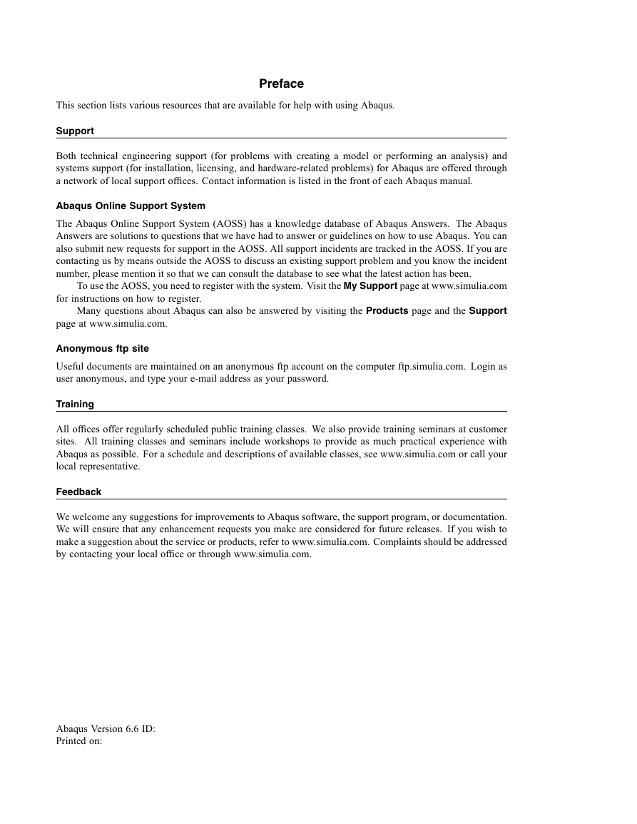
Preface
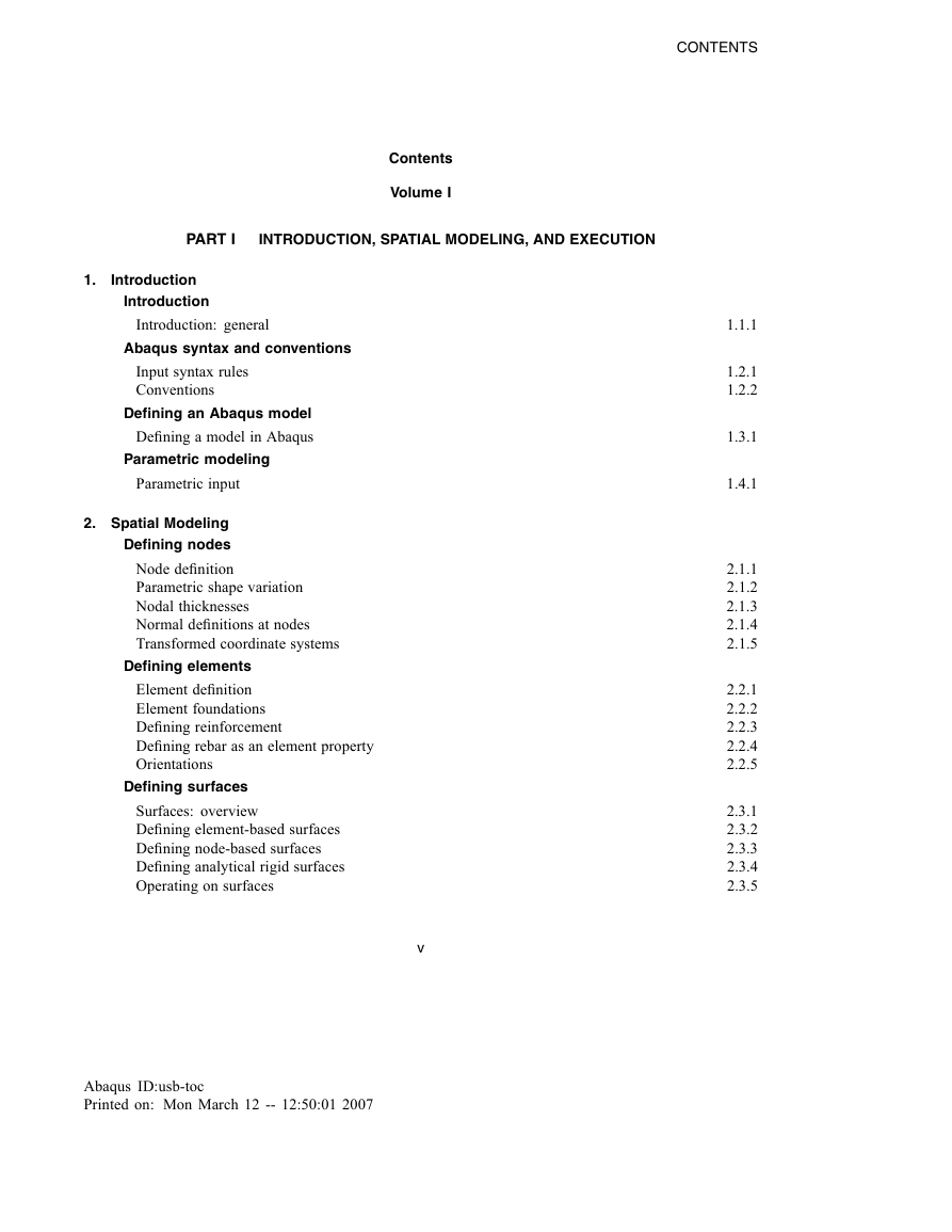
Contents
Part I: Introduction, Spatial Modeling, and Execution
1. Introduction
1.1 Introduction
1.1.1 Introduction: general
Overview of the Abaqus finite element system
Overview of this manual
Using Abaqus
Reviewing the results of an Abaqus simulation
1.2 Abaqus syntax and conventions
1.2.1 Input syntax rules
Overview
Keyword lines
Data lines
Sets
Labels
Repeating data lines
Example: Multiple data lines due to field variable dependence
Ordering the data lines
1.2.2 Conventions
Overview
Degrees of freedom
Axisymmetric elements
Activation of degrees of freedom
Internal variables in Abaqus/Standard
Coordinate systems
Units
Rotation and angle measures
International System of units (SI)
American or English units
Symbols used in Abaqus for units
Time
Local directions on surfaces in space
Rotation of the local directions
Convention used for stress and strain components
Nonisotropic material behavior
Zero-valued stress components
Shear strains
Stress and strain measures
Total (integrated) strain
Green's strain
Nominal strain
Logarithmic strain
Stress invariants
Finite rotations
Compound rotations
Example
1.3 Defining an Abaqus model
1.3.1 Defining a model in Abaqus
Overview
The input file
Model data
Required model data
Optional model data
History data
Required history data
Optional history data
Including model or history data from an external file
Including an encrypted data file
1.4 Parametric modeling
1.4.1 Parametric input
Overview
Introduction
Parameters
Independent parameters
Dependent parameters
Expressional dependence
Tabular dependence
Rules for parameters
Parameter evaluation
Parameter substitution
Data types
Continuous and discrete parameters
Auxiliary input files
Parametrization of input quantities
Parametrizing individual input quantities
Parametrizing groups of input quantities (expressional dependence)
Parametrizing groups of input quantities (tabular dependence)
Python language
Statement length and continuation lines
Comments
Parameter names
Data types
Type conversion
Numeric operators
Functions
Character string operators
Execution of parametrized input
Parameter check jobs
Display of parametric input
Data file display
Additional reference
2. Spatial Modeling
2.1 Defining nodes
2.1.1 Node definition
Overview
Assigning a node number to the node
Specifying a local coordinate system in which to define nodes
Defining the nodal coordinate system
Defining a nodal coordinate system within part definitions
Defining individual nodes by specifying their coordinates
Reading node definitions from a file
Specifying a local coordinate system for the nodal coordinates
Grouping nodes into node sets
Creating an unsorted node set
Assigning nodes to a node set as they are created
Assigning previously defined nodes to a node set
Listing the nodes that define the set directly
Generating the node set
Generating a node set from an element set
Limitation on updating node sets that are used to define other node sets
Defining part and assembly sets
Example
Alternate method for defining assembly-level node sets
Internal node sets created by Abaqus/CAE
Transferring of node sets
Creating nodes from existing nodes by generating them incrementally
Defining a straight line between the two end nodes
Defining a circular arc between the two end nodes
Defining a parabola between the two end nodes
Defining the extra point and the normal direction in a local coordinate system
Creating nodes by copying existing nodes
Translating and rotating the coordinates of the old nodes
Applying the rotation multiple times
Reflecting the coordinates of the old nodes
Reflecting the coordinates through a line
Reflecting the coordinates through a plane
Reflecting the coordinates through a point
Projecting the nodes in the old set from a pole node
Creating nodes by filling in nodes between two bounds
Example
Concentrating the nodes toward one bound or the other
Example
Applying the bias value at every second interval along the line
Creating quarter-point spacing
Example
Mapping a set of nodes from one coordinate system to another
Scaling the local coordinates before they are mapped
Specifying the scaling factors directly
Specifying the scaling with respect to a reference point
Introducing a simple shift and/or rotation by mapping from one coordinate system to another
Introducing a pure shift by specifying the axis and magnitude of the translation
Introducing a pure rotation by specifying the axis, origin, and angle of the rotation
Mapping from cylindrical coordinates
Mapping from skewed Cartesian coordinates
Mapping from spherical coordinates
Mapping from toroidal coordinates
Mapping by means of blended quadratics
2.1.2 Parametric shape variation
Overview
Parametrization of nodal coordinates
Direct parametrization of individual nodal coordinates
Parametrization of nodal coordinates using node generation
Shape change by linear combination of shape variations
Shape parametrization using shape variations
Defining shape variations directly or reading them from an alternate input file
Defining shape variations in alternative coordinate systems
Using auxiliary analyses to generate shape variations
Reading shape variations from a static analysis results file
Reading shape variations from an eigenvalue analysis results file
Shape parametrization and design sensitivity analysis
Visualization of shape variations
Using Abaqus/CAE to compute shape variations
2.1.3 Nodal thicknesses
Overview
Defining nodal thicknesses
Reading nodal thicknesses from an alternate file
Generating continuously varying thicknesses between two nodes or node sets
Specifying a continuously varying thickness for shell, membrane, and rigid elements
Specifying a continuously varying thickness for a composite shell
Example
Creating a discontinuity in the shell, membrane, or rigid element thicknesses
2.1.4 Normal definitions at nodes
Overview
Contact surfaces in Abaqus/Standard
Elements
Beam and shell elements
Line spring elements
Gasket elements
Contour integral evaluation
The coordinate system in which normals are defined
2.1.5 Transformed coordinate systems
Overview
Defining a local coordinate system
Defining a local coordinate system in a model that contains an assembly of part instances
Large-displacement analysis
Defining a rectangular Cartesian coordinate transformation
Defining a cylindrical coordinate transformation
Defining a spherical coordinate transformation
Output at a node associated with a coordinate transformation
2.2 Defining elements
2.2.1 Element definition
Overview
Assigning an element number to the element
Defining individual elements by specifying their nodes
Using large node numbers with elements that use many nodes
Reading element definitions from a file
Reading substructure definitions from a substructure library
Defining axisymmetric elements with asymmetric deformation
Defining gasket elements
Using solid element connectivity to define gasket elements
Examples
Defining cohesive elements
Defining a cohesive element by specifying all nodes
Defining a cohesive element by specifying only the bottom face nodes
Defining a pore pressure cohesive element by specifying only the bottom and top face nodes
Grouping elements into element sets
Assigning elements to an element set as they are created
Assigning previously defined elements to an element set
Listing the elements that form the set directly
Generating the element set
Limitation on updating element sets that are used to define other element sets
Defining part and assembly sets
Example
Alternate method for defining assembly-level element sets
Internal element sets created by Abaqus/CAE
Transferring of element sets
Creating elements from existing elements by generating them incrementally
Incrementing special-purpose nodes
Creating elements by copying existing elements
Special considerations for continuum elements
2.2.2 Element foundations
Overview
Defining element foundation behavior
2.2.3 Defining reinforcement
Overview
Defining a rebar layer
Assigning a name to the rebar layer
Specifying rebar geometry
Defining rebar with constant spacing
Defining rebar spacing as a function of radial position
Defining rebar using the tire “lift” equation
Local rebar orientation system
Local orientation system for three-dimensional elements
Local orientation system for axisymmetric elements
Large-displacement considerations
Defining rebar in Abaqus/Standard €beam elements
Defining the rebar material
Initial conditions
Defining prestress in rebar
Holding prestress in rebar in Abaqus/Standard
Defining the initial values of solution-dependent state variables for rebars
Output
Specifying the direction for rebar angle output
Example
Visualizing rebar orientation and results in rebar
2.2.4 Defining rebar as an element property
Overview
Assigning a name to the rebar set
Defining rebars in three-dimensional shell and membrane elements
Defining isoparametric rebars in three-dimensional shell and membrane elements
Defining skew rebars in three-dimensional shell and membrane elements
Defining skew rebars relative to the default projected local coordinate system
Defining skew rebars relative to a user-defined local coordinate system
Defining rebars in axisymmetric shell and membrane elements
Defining rebars in continuum elements
Defining layers of rebars in planar and axisymmetric continuum elements
Defining isoparametric rebars
Defining skew rebars
Defining single rebars in two-dimensional axisymmetric and generalized plane strain continuum elements
Defining layers of rebars in three-dimensional continuum elements
Defining isoparametric rebars
Example: isoparametric rebar
Defining skew rebars
Example: skew rebar
Defining single rebars in three-dimensional continuum elements
Defining the rebar material
Initial conditions
Defining prestress in rebar
Holding prestress in rebar in Abaqus/Standard
Defining the initial values of solution-dependent state variables for rebars
Output
Specifying the direction for rebar angle output in shell and membrane elements
Example
Visualizing rebar orientation and results in rebar
2.2.5 Orientations
Overview
Assigning a name to an orientation
Defining a local coordinate system in a model that contains an assembly of part instances
Defining a local coordinate system directly
Available coordinate systems
Defining a rectangular coordinate system
Defining a cylindrical coordinate system
Defining a spherical coordinate system
Methods for defining a coordinate system
Defining a coordinate system by specifying the locations of points a, b, and c directly
Defining a coordinate system by giving global node numbers for points a, b, and c
Defining a coordinate system by giving local node numbers for points a, b, and c
Defining a coordinate system by giving an offset from another coordinate system
Defining a coordinate system by giving two edges
Defining a local coordinate system in Abaqus/Standard €using a user subroutine
Multiple references to an orientation definition
Large-displacement considerations
Use with two-dimensional solid elements
Use with shell, membrane, or gasket elements or contact surfaces
Defining rebars in shell, membrane, and surface elements
Special considerations when defining orientations on contact surfaces in Abaqus/Standard
Use with laminated shells
Use with laminated three-dimensional solid elements
Use with pipe-soil interaction elements
Use with beam, frame, and truss elements
Use with the jointed material model
Use with rotary inertia and connector elements
Use with the kinematic coupling constraint
Use with surface-based coupling constraints
Use with inertia relief
Use with distributed general traction, shear traction, and general edge loads
Orientations defined with distributions
Output
2.3 Defining surfaces
2.3.1 Surfaces: overview
Overview
Why use surfaces?
Internal surfaces created by Abaqus/CAE
Restrictions on surfaces
2.3.2 Defining element-based surfaces
Overview
Defining element-based surfaces
General restrictions on element-based surfaces
Surface discretization
Creating surfaces on solid, continuum shell, and cohesive elements
Generating the free surface automatically
Special treatment of cohesive elements for automatic free surface generation
Creating surface facets by specifying solid, continuum shell, and cohesive element faces
Generating an interior surface automatically
Creating surfaces on structural, surface, and rigid elements
Defining single-sided surfaces
Defining double-sided surfaces
Defining edge-based surfaces
Defining a surface over the cross-section at the ends of beam, pipe, and truss elements
Defining a surface along the length of three-dimensional beam, pipe, and truss elements
Surfaces along the length of two-dimensional beam and truss elements
Shell, membrane, or rigid element thickness and shell offset
Creating surfaces on gasket elements
Surfaces on three-dimensional gasket line elements
Creating interior cross-section surfaces
Whole-model free surface in an Abaqus/Explicit input file
Trimming the perimeter of an open surface
The effect of surface trimming
Why Abaqus will, by default, trim most surfaces
2.3.3 Defining node-based surfaces
Overview
Creating a node-based surface
2.3.4 Defining analytical rigid surfaces
Overview
What are analytical rigid surfaces and why use them?
Advantages
Disadvantages
Creating an analytical rigid surface
Defining a surface profile
Two-dimensional rigid surfaces
Three-dimensional cylindrical rigid surfaces
Three-dimensional surfaces of revolution
Defining the surface normals
Smoothing analytical rigid surfaces
Surface tangent conventions
Creating an analytical rigid surface in a user subroutine
Defining analytical rigid surfaces when drag chain or rigid surface elements are used
Two-dimensional rigid surfaces
Three-dimensional cylindrical rigid surfaces
2.3.5 Operating on surfaces
Overview
Creating a combined surface
Union of existing surfaces
Intersection or difference of existing surfaces
Creating a cropped surface
2.4 Defining rigid bodies
2.4.1 Rigid body definition
Overview
What is a rigid body?
Determining when to use a rigid body
Creating a rigid body
The rigid body reference node
Positioning the reference node at the center of mass
The collection of nodes that constitute the rigid body
Assigning elements to a rigid body
Assigning nodes to a rigid body
Assigning analytical surfaces to a rigid body
Defining a rigid body in a model that is defined in terms of an assembly of part instances
Rigid body mass and inertial properties
Defining mass and inertia properties by discretization
Defining mass and inertia properties directly
Kinematics of a rigid body
Rigid body motions
Boundary conditions
Constraints
Connector elements
Planar rigid body
Axisymmetric rigid body
Three-dimensional rigid body
Defining loads on rigid bodies
Rigid bodies with temperature degrees of freedom
Modeling contact with a rigid body
Limitations in Abaqus/Standard
Limitations in Abaqus/Explicit
Using rigid bodies in geometrically linear Abaqus/Standard €analysis
2.5 Defining integrated output sections
2.5.1 Integrated output section definition
Overview
Introduction
Creating an integrated output section
Creating interior cross-section surfaces
The integrated output section reference node
Positioning the reference node at the center of the surface
Setting the reference node to track the average motion of the surface
The integrated output section local coordinate system
Projecting the coordinate system onto the section surface
Associating an integrated output section with an integrated output request
Limitations
2.6 Defining nonstructural mass
2.6.1 Nonstructural mass definition
Overview
Nonstructural mass
Defining nonstructural mass
Specifying the units of the nonstructural mass
Specifying units of mass
Specifying units of mass per unit volume
Specifying units of mass per unit area
Specifying units of mass per unit length
Controlling the distribution of the total mass from nonstructural features
Distributing the nonstructural mass in proportion to the element structural mass
Distributing the nonstructural mass in proportion to the element volume
2.7 Defining distributions
2.7.1 Distribution definition
Overview
Distributions
Specifying the location of a distribution
Defining a distribution on elements
Defining a distribution on nodes
Defining a distribution table
Applying distributions
Examples
Example 1
Example 2
Example 3
2.8 Defining display bodies
2.8.1 Display body definition
Overview
What is a display body?
Creating a display body
The reference nodes
Using display bodies with connectors
Input file template
2.9 Defining an assembly
2.9.1 Defining an assembly
Overview
Introduction
Terminology
Example
Defining parts, part instances, and the assembly
Defining a part
Defining part instances
Defining the assembly
Example
Notes
Organizing the model definition
Rules for defining an assembly
Referring to items between levels
Naming conventions
Quoted labels
Example
The mesh (nodes and elements)
Section definitions
Sets and surfaces
Defining assembly-level sets
Adding sets and surfaces on restart
Rigid bodies
Materials
Interactions
Constraints
Examples
Coordinate system definitions
Translating and rotating a part instance
Limitations
Input file template
2.10 Defining matrices
2.10.1 Defining matrices
Overview
What is a matrix in Abaqus/Standard ?
Including matrices in a model
Scaling the matrix data
Reading the matrix data from an alternate file
Defining the stiffness and mass with matrices included in a model
Connecting a part of a model represented by matrices
Using matrices in static analysis
Using matrices in a natural frequency extraction analysis
Constraints and transformations
Initial conditions
Boundary conditions
Loads
Elements
Output
Limitations
Input file template
3. Execution Procedures
3.1 Execution procedures: overview
3.1.1 Execution procedure for Abaqus: overview
Overview
Conventions
Environment settings
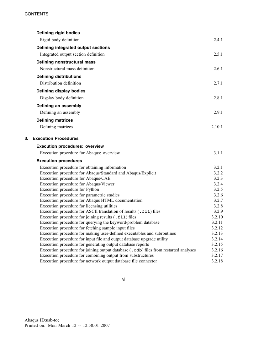
3.2 Execution procedures
3.2.1 Execution procedure for obtaining information
Overview
Command summary
Command line options
Examples
3.2.2 Execution procedure for Abaqus/Standard and Abaqus/Explicit
Overview
Command summary
Command line options
Required option
Mutually exclusive options that determine which phases of an analysis are performed
Additional options available for the analysis module
Examples
Running analyses in Abaqus/Standard
Running analyses in Abaqus/Explicit
Running different phases of an analysis
Running a co-simulation using Abaqus and AcuSolve
Running a co-simulation using Abaqus/Explicit and MADYMO
3.2.3 Execution procedure for Abaqus/CAE
Overview
Command summary
Command line options
Examples
Opening a model database
Passing arguments to a script
Running Abaqus/CAE without the graphical user interface
3.2.4 Execution procedure for Abaqus/Viewer
Overview
Command summary
Command line options
3.2.5 Execution procedure for Python
Overview
Command summary
Command line option
3.2.6 Execution procedure for parametric studies
Overview
Command summary
Command line options
Examples
3.2.7 Execution procedure for Abaqus HTML documentation
Overview
Using Abaqus HTML documentation
Command summary
3.2.8 Execution procedure for licensing utilities
Overview
Command summary
Command line options
3.2.9 Execution procedure for ASCII translation of results ( .fil ) files
Overview
Command summary
Command line options
Example
3.2.10 Execution procedure for joining results ( .fil ) files
Overview
Command summary
Command line options
Example
3.2.11 Execution procedure for querying the keyword/problem database
Overview
Command summary
Command line options
Examples
Querying for keywords and parameters
Querying for user-specified parameter values
3.2.12 Execution procedure for fetching sample input files
Overview
Command summary
Command line options
Examples
3.2.13 Execution procedure for making user-defined executables and subroutines
Overview
Command summary
Command line options
Example
3.2.14 Execution procedure for input file and output database upgrade utility
Overview
Command summary
Command line options
Required option
Mutually exclusive options
Additional options
3.2.15 Execution procedure for generating output database reports
Overview
Output database structure
Generating summary reports
Adding information to a report
Additional options
Command summary
Command line options
Required options
File formatting option
Option to generate a full output database report
Options to report model data
Options to report results data
Options to report field output variables
Options to report different field variable attributes
Options to report history output variables
Additional options
Examples
File naming and formatting
Adding information to a report
Additional options
Selecting frames
3.2.16 Execution procedure for joining output database ( .odb ) files from restarted analyses
Overview
Appending data when the analysis restarts between steps versus midstep
Customizing the combined output database file
Command summary
Command line options
Examples
3.2.17 Execution procedure for combining output from substructures
Overview
Combining data for models with more than two substructures
Customizing the combined output database
Command summary
Command line options
Examples
Combining two substructures
Combining more than two substructures
Combining specific elements of the substructures
3.2.18 Execution procedure for network output database file connector
Overview
Command summary
Command line options
3.2.19 Execution procedure for fixed format conversion utility
Overview
Command summary
Command line options
3.2.20 Execution procedure for translating NASTRAN bulk data files to Abaqus input files
Overview
Using the translator
Summary of NASTRAN entities translated
Command summary
Command line options
3.2.21 Execution procedure for translating PAM-CRASH input files to partial Abaqus input files
Overview
Using the translator
Element numbering and grouping
Material models
History section data
Summary of PAM-CRASH entities translated
Command summary
Command line options
3.2.22 Execution procedure for translating RADIOSS input files to partial Abaqus input files
Overview
Using the translator
Element numbering and grouping
Material models
Summary of RADIOSS entities translated
Command summary
Command line options
3.2.23 Execution procedure for translating Abaqus output database files to NASTRAN Output2 results files
Overview
Using the translator
Command summary
Command line options
3.2.24 Execution procedure for exchanging Abaqus data with ZAERO
Overview
Universal file
Preparing the Abaqus analysis input file
Workflow
Modal analysis in Abaqus
Aeroelastic analysis in ZAERO
Stress analysis in Abaqus
Command summary
Command line options
3.2.25 Execution procedure for encrypting and decrypting Abaqus input data
Overview
Specifying additional access levels and controls
Security and support considerations
Adding comments to the header of an encrypted file
Command summary
Command line options
Examples
Creating encrypted files
Limiting access to decrypted files by license feature or site ID
Creating encrypted files that must be included to be used by Abaqus
3.2.26 Execution procedures for job execution control
Overview
Command summary
Command line options
Required option
3.3 Environment file settings
3.3.1 Using the Abaqus environment settings
Overview
Environment settings hierarchy
Syntax
Troubleshooting
Command line default parameters
System resource parameters
System customization parameters
Scratch file management parameters
Co-simulation parameters
Environment file examples
UNIX environment file:
Windows environment file:
3.4 Managing memory and disk resources
3.4.1 Managing memory and disk use in Abaqus
Overview
Understanding resource use
Abaqus data
Requirements and considerations
Resource management parameters
Memory management parameters
Disk management parameters
Units
Input file processing
Guidelines for memory settings
Setting pre_memory on single-user machines
Setting pre_memory on multi-user machines
Setting pre_memory when using queues
Abaqus/Standard analysis
Memory management
The standard_memory parameter
The standard_memory_policy parameter
Guidelines for memory settings
Setting standard_memory on single-user machines
Setting standard_memory on multi-user machines
Setting standard_memory when using queues
Setting standard_memory_policy
Examples
Scratch file management
General scratch file management parameters
Determining when to split files
Example: Splitting the factor ( .fct ) file
Parallel Lanczos scratch file management
3.5 File extension definitions
3.5.1 File extensions used by Abaqus
Overview
File extensions
3.6 FORTRAN unit numbers
3.6.1 FORTRAN unit numbers used by Abaqus
Overview
FORTRAN unit numbers
Part II: Output
4. Output
4.1 Output
4.1.1 Output
Overview
The data file
Controlling the amount of analysis input file processor information written to the data file
Input file echo
Input parameter information
Parameter-free input file information
Model and history definition summaries
Contact constraint information
Requesting printed results
Viewing part and assembly information in the data file
The output database
Requesting output to the output database
Format of the output database
The selected results file
The results file
Obtaining results file output in Abaqus/Standard
Obtaining results at the beginning of a step
Obtaining results file output in Abaqus/Explicit
Part and assembly information
Format of the results file
Controlling the format of the results file in Abaqus/Standard
Controlling the format of the results file in Abaqus/Explicit
ASCII format
Precision of floating point data in the results file
Maximizing the efficiency of the results file
Example
The message file
The Abaqus/Standard message file
Controlling the frequency of output to the message file
Requesting detailed contact printout
Requesting detailed model change printout
Requesting detailed printout of problems with the plasticity algorithms
Requesting output of equilibrium residuals
Requesting solver information
Requesting detailed adaptive mesh smoothing printout
Monitoring a degree of freedom in the message file
The Abaqus/Explicit message file
The status file
The Abaqus/Standard status file
The Abaqus/Explicit status file
Requesting kinetic energy output
Requesting total energy output
Requesting output of the critical element
Requesting output of the change in the total mass
Monitoring a degree of freedom in the status file
Requesting output in multiple steps
General analysis steps
Linear perturbation steps
Element matrix output in Abaqus/Standard
Writing the element matrices to the results file
Writing the element matrices to a user-defined file
Writing the element matrices to the data file
Including distributed loads
Controlling the frequency of element matrix output
Writing the stiffness or operator matrix
Writing the mass matrix
User-defined output variables in Abaqus/Standard
User-defined state variables in Abaqus/Standard
Postprocessing with Abaqus/CAE
Recovering additional results output from restart data in Abaqus/Standard
Recovering additional output from a direct cyclic analysis
Example
4.1.2 Output to the data and results files
Overview
Requesting output to the data and results files
Output to the Abaqus/Standard data file
Output to the Abaqus/Standard results file
Output to the Abaqus/Explicit results file
Output frequency
Element output
Selecting the element output variables
Selecting the elements for which output is required
Specifying the section point in beams, shells, and layered solid elements
Requesting output for rebars in a reinforced model
Selecting the position of element integration and section point output in Abaqus/Standard
Obtaining element output at the integration points
Obtaining element output at the centroid of each element
Obtaining element output averaged at the nodes
Obtaining element output extrapolated to the nodes
Extrapolation and interpolation of element output variables
Requesting summaries in the Abaqus/Standard data file
Requesting totals in the Abaqus/Standard data file
Controlling the frequency of output
Specifying the directions for element output
Controlling the output during eigenvalue extraction
Abaqus/Standard data file format
Results file format
Output of local directions to the results file
Default element output
Node output
Selecting the nodal output variables
Selecting the nodes for which output is required
Requesting summaries in the Abaqus/Standard data file
Requesting totals in the Abaqus/Standard data file
Controlling the frequency of output
Specifying the directions for nodal output
Obtaining nodal output in the global directions
Obtaining nodal output in the local directions defined by nodal transformations
Controlling the output during eigenvalue extraction
Abaqus/Standard data file format
Results file format
Default nodal output
Total energy output
Selecting the energy output variables
Selecting the element set for which total energy output is required
Controlling the frequency of output
Default energy output
Modal output from Abaqus/Standard
Selecting the modal output variables
Controlling the frequency of output
Default modal output
Surface output from Abaqus/Standard
Selecting the surface output variables
Selecting the contact pairs for which output is required
Requesting summaries in the data file
Requesting totals in the data file
Controlling the frequency of output
Default surface output
Data file format
Results file format
Fastener interaction output from Abaqus/Standard
Selecting the fastener interaction output variables
Selecting the fastener interactions for which output is required
Requesting summaries in the data file
Requesting totals in the data file
Controlling the frequency of output
Default fastener interaction output
Data file format
Section output from Abaqus/Standard
Defining the surface section
Example
Selecting the coordinate system in which output is desired
Defining a coordinate system local to the surface section
Default local system
User-specified local system
Controlling the frequency of output
Data file format
Results file format
Vector output in the section
Scalar output in the section
Limitations when using section output requests
4.1.3 Output to the output database
Overview
Requesting output to the output database
Requesting field output
Requesting history output
Requesting diagnostic information
Controlling the output frequency
Controlling the output frequency in Abaqus/Standard
Specifying output frequency in increments
Specifying output frequency in number of intervals
Specifying output frequency in regular time interval size
Specifying output frequency in time points
Time incrementation
Default output
Controlling the output frequency for field output in Abaqus/Explicit
Specifying field output frequency in number of intervals
Specifying field output frequency in regular time interval size
Specifying field output frequency in time points
Default field output
Controlling the output frequency for history output in Abaqus/Explicit
Specifying history output frequency in increments
Specifying history output frequency in regular time interval size
Default history output
Requesting output in multiple steps
Specifying new output requests
Specifying additional output requests
Replacing or removing an output request
Suppressing output requests defined in previous steps
Preselected output requests
Requesting procedure-specific preselected output requests
Requesting all variables applicable to the current procedure and material type
Default output
Abaqus/Explicit output as a result of analysis termination
Selecting eigenmodes desired for output in Abaqus/Standard
Element output
Selecting the element output variables
Selecting elements for which output is required
Specifying the section point in beam, shell, and layered solid elements
Requesting output for rebars in a reinforced model
Selecting the position of element integration point and section point output
Obtaining output at the integration points
Obtaining output at the centroid of each element
Obtaining element output extrapolated to the nodes
Extrapolation and interpolation of element output variables
Controlling the output frequency
Requesting preselected output
Specifying the directions for element output
Node output
Selecting the nodal output variables
Selecting the nodes for which output is required
Controlling the output frequency
Controlling the precision
Requesting preselected output
Specifying the directions for nodal output
Visualizing boundary conditions
Tracer particle output from Abaqus/Explicit
Defining tracer particles
Particle birth stages
Tracer particles in the output database
Requesting output at tracer particles
Field output at tracer particles
History output at tracer particles
Tracer particle propagation in multiple steps
Tracer particle deactivation
Controlling the output frequency at tracer particles
Integrated output in Abaqus/Explicit
Selecting the integrated output variables
Selecting the surface over which integrated output is required
Specifying the surface for integrated output directly
Specifying the surface through an integrated output section definition
Requesting integrated output for “force-flow” studies
Requesting integrated output over an element set
Controlling the output frequency
Requesting preselected output
Limitations when using integrated output requests
Total energy output
Selecting the energy output variables
Selecting the element set for which total energy output is required
Controlling the output frequency
Requesting preselected output
Filtering history output in Abaqus/Explicit
Defining a low-pass Infinite Impulse Response filter
Start-up conditions for the filter
Filtering using the low-pass Infinite Impulse Response filters
Filtering the output based on the sampling interval
Modal output from Abaqus/Standard
Selecting the modal output variables
Controlling the frequency of output
Requesting output
Surface output
Selecting the surface output variables
Selecting the contact pairs for which output is required in Abaqus/Standard
Selecting the contact pairs for which output is required in Abaqus/Explicit
Selecting output for general contact interactions in Abaqus/Explicit
Field output
History output
Controlling the output frequency
Requesting preselected output
Time incrementation output in Abaqus/Explicit
Selecting the incrementation output variables
Controlling the output frequency
Requesting preselected output
Fastener interaction output
Selecting the fastener interaction output variables
Selecting the fastener interactions for which output is required
Controlling the output frequency
Requesting preselected output
Cavity radiation output in Abaqus/Standard
Selecting the radiation output variables
Selecting the region of the model for which radiation output is required
Controlling the output frequency
Requesting output
Examples
Abaqus/Standard example
Abaqus/Explicit example
4.2 Output variables
4.2.1 Abaqus/Standard output variable identifiers
Overview
Symbols used in the tables
Requesting output of components
Direction definitions
Direction definitions for element variables
Direction definitions for equivalent rigid body variables
Direction definitions for nodal variables
Direction definitions for integrated variables
Strain output
Temperature output
Principal value output
Tensor output
Element integration point variables
Tensors and associated principal values and invariants
Additional element stresses
Vibration and acoustic quantities
Energy densities
State, field, and user-defined output variables
Composite failure measures
Fluid link quantities
Fracture mechanics quantities
Concrete cracking and additional plasticity
Concrete damaged plasticity
Rebar quantities
Heat transfer analysis
Mass diffusion analysis
Elements with electrical potential degrees of freedom
Piezoelectric analysis
Coupled thermal-electrical elements
Cohesive elements
Pore pressure analysis
Pore pressure cohesive elements
Porous metal plasticity quantities
Two-layer viscoplasticity quantities
Geometric quantities
Accuracy indicators
Random response analysis
Steady-state dynamic analysis
Fiber reinforced materials damage
Element section variables
Frame elements
Whole element variables
Connector elements
Element face variables
Whole element energy density variables
Whole element error indicator variables
Nodal variables
Acoustic quantities
Heat or mass flux
Steady-state dynamic analysis
Modal dynamic, steady-state, and random response analysis
Mode-based steady-state dynamic analysis
Pore pressure analysis
Random response analysis
Modal variables
Surface variables
Mechanical analysis–nodal quantities
Mechanical analysis–whole surface quantities
Heat transfer analysis
Coupled thermal-electrical analysis
Fully coupled temperature-displacement analysis
Coupled pore fluid-mechanical analysis–nodal quantities
Coupled pore fluid-mechanical analysis–whole surface quantities
Bond failure quantities
Cavity radiation variables
Section variables
All analysis types
Stress/displacement analysis
Heat transfer analysis
Electrical analysis
Mass diffusion analysis
Coupled pore fluid diffusion-stress analysis
Fastener interaction variables
Whole and partial model variables
Adaptive mesh domains
Equivalent rigid body motion variables
Inertia relief output variables
Mass diffusion analysis
Eigenvalue extraction
Complex eigenvalue extraction
Total energy output quantities
Solution-dependent amplitude variables
4.2.2 Abaqus/Explicit output variable identifiers
Overview
Symbols used in the tables
Direction definitions
Direction definitions for element variables
Direction definitions for nodal variables
Direction definitions for integrated variables
Principal value output
Tensor output
Requesting output of components
Element integration point variables
Tensors and invariants
Additional element stresses
Energy densities
State and field variables
Composite failure measures
Additional plasticity quantities
Porous metal plasticity quantities
Concrete damaged plasticity
Cracking model quantities
Failure with progressive damage
Fiber-reinforced materials damage
Equation of state
Rebar quantities
Integration point coordinates
Coupled thermal-stress elements
Cohesive elements
Element section variables
Whole element variables
Connector elements
Element face variables
Nodal variables
Fluid cavity variables
Surface variables
Mechanical analysis–nodal quantities
Mechanical analysis–whole surface quantities
Fully coupled temperature-displacement analysis
Fastener interaction variables
Integrated variables
Total energy output
Time increment and mass output
4.3 The postprocessing calculator
4.3.1 The postprocessing calculator
Overview
Functionality of the calculator
Running the calculator
5. File Output Format
5.1 Accessing the results file
5.1.1 Accessing the results file: overview
Writing information to the results file
Accessing information in the results file
5.1.2 Results file output format
Overview
Record format
Local coordinate system
Label record
Records written for any file output request
Record written once per eigenvalue in natural frequency extraction
Records written once per increment
Records written for any element file output request
Principal value records
Records for porous metal plasticity
Records for brittle cracking
Records for inelastic nonlinear response in a beam general section
Records for elastic-plastic response in frame elements
Records for connector elements
Record for plane stress orthotropic failure measures
Record for equivalent plastic strain components for cap plasticity
Record for equivalent plastic strain components for jointed materials
Record for equivalent plastic strain in uniaxial tension for cast iron plasticity
Records for two-layer viscoplasticity
Record for elements with electric potential degrees of freedom
Records for rebar quantities
Record for forced convection/diffusion heat transfer elements
Records for piezoelectric materials
Records for coupled thermal-electric elements
Records for equivalent rigid body variables in direct-integration implicit dynamic analyses
Record for transverse shear stress in thick shell elements such as S3R, S4R, S8R, and S8RT
Records for linear dynamics
Records for connector elements (available only for linear dynamics)
Records for fluid link elements (available only for linear dynamics)
Records for output of element volumes
Record for solid elements in an adaptive mesh domain in Abaqus/Standard
Records written for any node file output request
Records for linear dynamics
Records written for any modal file output request during mode-based dynamic analysis
Records written for any element matrix or substructure matrix file output request
Record written for any energy file output request
Records written for contour integrals
Record written for crack propagation analysis
Records written once for any file output request when surfaces are defined in Abaqus/Standard
Rigid surfaces
Deformable surfaces
Records written for any contact surface file output request
Records for bond failure quantities from crack propagation analysis
Record for surface-based pressure penetration analysis
Records written once for any file output request when cavities are defined
Records written for any viewfactor matrix output request
Records written for any radiation file output request
Records written for any section file output request
For all analysis types
For stress/displacement analyses
For heat transfer analyses
For electrical analyses
For mass diffusion analyses
For coupled pore fluid diffusion-stress analyses
Procedure type keys
5.1.3 Accessing the results file information
Overview
Reading floating point and integer variables
Linking the postprocessing program
Calling the utility subroutines for reading the results file
Example
Writing a file in the results file format
5.1.4 Utility routines for accessing the results file
Overview
DBFILE (read from a file)
Interface
Variable to be provided to the utility routine
Variables returned from the utility routine
DBFILW (write to a file)
Interface
Variables to be provided to the utility routine
DBRNU (set a unit number for a file)
Interface
Variable to be provided to the utility routine
INITPF (initialize a file)
Interface
Variables to be provided to the utility routine
File naming conventions
POSFIL (determine position in a file)
Interface
Variables to be provided to the utility routine
Variables returned from the utility routine
Positioning with POSFIL
Examples
OI.1 Abaqus/Standard Output Variable Index
OI.2 Abaqus/Explicit Output Variable Index



 2023年江西萍乡中考道德与法治真题及答案.doc
 2012年重庆南川中考生物真题及答案.doc
 2013年江西师范大学地理学综合及文艺理论基础考研真题.doc
 2020年四川甘孜小升初语文真题及答案I卷.doc
 2020年注册岩土工程师专业基础考试真题及答案.doc
 2023-2024学年福建省厦门市九年级上学期数学月考试题及答案.doc
 2021-2022学年辽宁省沈阳市大东区九年级上学期语文期末试题及答案.doc
 2022-2023学年北京东城区初三第一学期物理期末试卷及答案.doc
 2018上半年江西教师资格初中地理学科知识与教学能力真题及答案.doc
 2012年河北国家公务员申论考试真题及答案-省级.doc
 2020-2021学年江苏省扬州市江都区邵樊片九年级上学期数学第一次质量检测试题及答案.doc
 2022下半年黑龙江教师资格证中学综合素质真题及答案.doc