20年单类别(One-Class)分类全面综述论文.pdf

发布时间：2022-05-31 发布人：admin 分类：说明书资料大小：3.91M 资料格式：pdf 举报版权申诉

syp_net-14803622-16359647455062601643.pdf-第1页.png

第1页 / 共19页

syp_net-14803622-16359647455062601643.pdf-第2页.png

第2页 / 共19页

syp_net-14803622-16359647455062601643.pdf-第3页.png

第3页 / 共19页

syp_net-14803622-16359647455062601643.pdf-第4页.png

第4页 / 共19页

syp_net-14803622-16359647455062601643.pdf-第5页.png

第5页 / 共19页

syp_net-14803622-16359647455062601643.pdf-第6页.png

第6页 / 共19页

syp_net-14803622-16359647455062601643.pdf-第7页.png

第7页 / 共19页

syp_net-14803622-16359647455062601643.pdf-第8页.png

第8页 / 共19页

I Introduction

II Taxonomy

III Features for OCC

III-A Statistical Features

III-B Deep learning-based Features

IV OCC Algorithms

IV-A Representation-based Methods

IV-B Statistical Methods

IV-C Deep Learning Methods

IV-C1 Discriminative Methods

IV-C2 Generative Models

IV-C3 Knowledge Distillation

V Datasets and Evaluation Protocols

V-A Multi-class Benchmark Datasets

V-B Abnormal 1001 Dataset

V-C MVTec-AD Dataset

V-D Evaluation Metrics

VI Discussion and future research directions

References

One-Class Classiﬁcation: A Survey Pramuditha Perera, Member, IEEE, Poojan Oza, Student Member, IEEE and Vishal M. Patel, Senior Member, IEEE 1 1 2 0 2 n a J 8 ] V C . s c [ 1 v 4 6 0 3 0 . 1 0 1 2 : v i X r a Abstract—One-Class Classiﬁcation (OCC) is a special case of multi-class classiﬁcation, where data observed during training is from a single positive class. The goal of OCC is to learn a representation and/or a classiﬁer that enables recognition of positively labeled queries during inference. This topic has received considerable amount of interest in the computer vision, machine learning and biometrics communities in recent years. In this article, we provide a survey of classical statistical and recent deep learning-based OCC methods for visual recognition. We discuss the merits and drawbacks of existing OCC approaches and identify promising avenues for research in this ﬁeld. In addition, we present a discussion of commonly used datasets and evaluation metrics for OCC. I. INTRODUCTION Over the last decade, methods based on Deep Convolutional Neural Networks (DCNNs) have shown impressive perfor- mance improvements for object detection and recognition problems. Availability of large multi-class annotated datasets makes it possible for deep networks to learn discriminative features that a classiﬁer can exploit to perform recognition. In this survey we focus on the extreme case of recognition – One-Class Classiﬁcation (OCC), where data from only a single class (labeled positive) is present during training. During infer- ence, the classiﬁer encounters data from both the positive class and outside the positive class (sometimes referred to as the negative class). The objective of OCC is to determine whether a query object belongs to the class observed during training. In the absence of multiple-class data, both learning features and deﬁning classiﬁcation boundaries become more challenging in OCC compared to multi-class classiﬁcation. Nevertheless, it has applications in several image-based machine learning tasks. One-class classiﬁcation methods are extensively used in abnormal image detection [70], [8] and abnormal event detec- tion [87], [41]. They are also used extensively in biometrics applications such as Active Authentication [63], [56] and anti- spooﬁng [22], [54], [20], [99]. Therefore, there has been a signiﬁcant interest in the computer vision, machine learning and biometrics communities in developing OCC algorithms. 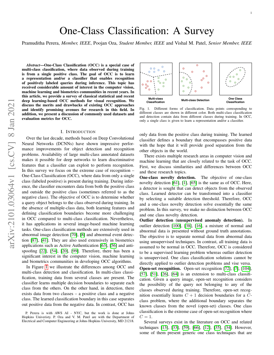In Figure 1 we illustrate the differences among OCC and multi-class detection and classiﬁcation. In multi-class classi- ﬁcation, training data from several classes are present. The classiﬁer learns multiple decision boundaries to separate each class from the others. On the other hand, in detection, there exists data from two classes – a positive class and a negative class. The learned classiﬁcation boundary in this case separates out positive data from the negative data. In contrast, OCC has P. Perera is with AWS AI - NYC, but the work is done at Johns Hopkins Univeristy. P. Oza and V. M. Patel are with the Department of Electrical and Computer Engineering at Johns Hopkins University, MD 21218. Fig. 1. Different forms of classiﬁcation. Data points corresponding to different classes are shown in different color. Both multi-class classiﬁcation and detection contain data from different classes during training. In OCC, only a single class is given to learn a representation and/or a classiﬁer. only data from the positive class during training. The learned classiﬁer deﬁnes a boundary that encompasses positive data with the hope that it will provide good separation from the other objects in the world. There exists multiple research areas in computer vision and machine learning that are closely related to the task of OCC. First, we discuss similarities and differences between OCC and these research topics. One-class novelty detection. The objective of one-class novelty detection [61], [1], [65] is the same as of OCC. Here, a detector is sought that can detect objects from the observed class. Learned detector can be transformed into a classiﬁer by selecting a suitable detection threshold. Therefore, OCC and a one-class novelty detection solve essentially the same problem. In this survey, we make no distinction between OCC and one class novelty detection. Outlier detection (unsupervised anomaly detection). In outlier detection [100], [38], [16], a mixture of normal and abnormal data is presented without ground truth annotations. The objective is to separate normal data from abnormal data using unsupervised techniques. In contrast, all training data is assumed to be normal in OCC. Therefore, OCC is considered to be a supervised learning problem whereas outlier detection is unsupervised. One class classiﬁcation solutions cannot be directly applied to outlier detection problems and vise versa. Open-set recognition. Open-set recognition [72], [7], [104], [57], [51], [26], [64] is an extension to multi-class classiﬁ- cation. Given a query image, open-set recognition considers the possibility of the query not belonging to any of the classes observed during training. Therefore, open-set recog- nition essentially learns C + 1 decision boundaries for a C- class problem, where the additional boundary separates the known classes from the novel (open-set) classes. One class classiﬁcation is the extreme case of open-set recognition where C = 1. Several surveys exist in the literature on OCC and related techniques [13], [33], [59], [66], [12], [35], [34]. However, some of them present generic one class techniques that are Multi-classClassiﬁcationMulti-class DetectionOne ClassClassiﬁcation

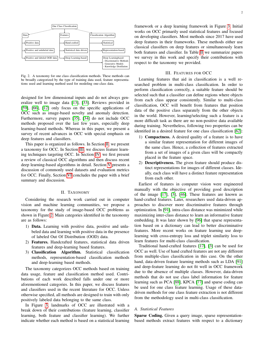
One Class Classiﬁcation Data Features Classiﬁcation Algorithm Positive data Hand-crafted Statistical Positive and unlabeled data Statistical data driven Representation-based Positive and labeled OOD data Deep Learning-based Deep Learningbased: - Discriminative Methods - Generative Models - Knowledge Distillation Fig. 2. A taxonomy for one class classiﬁcation methods. These methods can be broadly categorized by the type of training data used, feature representa- tions used and learning method used for modeling one-class data. designed for low dimensional inputs and do not always gen- eralize well to image data [13], [33]. Reviews provided in [59], [66], [12] only focus on the speciﬁc applications of OCC such as image-based novelty and anomaly detection. Furthermore, survey papers [35], [34] do not include OCC methods proposed over the last few years, especially deep learning-based methods. Whereas in this paper, we present a survey of recent advances in OCC with special emphasis on deep features and classiﬁers. This paper is organized as follows. In Section II, we present a taxonomy for OCC. In Section III, we discuss feature learn- ing techniques targeting OCC. In Section IV, we ﬁrst present a review of classical OCC algorithms and then discuss recent deep learning-based algorithms in detail. Section V presents a discussion of commonly used datasets and evaluation metrics for OCC. Finally, Section VI concludes the paper with a brief summary and discussion. II. TAXONOMY Considering the research work carried out in computer vision and machine learning communities, we propose a taxonomy for the study of image-based OCC problems as shown in Figure 2. Main categories identiﬁed in the taxonomy are as follows: 1) Data. Learning with positive data, positive and unla- beled data and learning with positive data in the presence of labeled Out Of Distribution (OOD) data. 2) Features. Handcrafted features, statistical data driven features and deep-learning based features. 3) Classiﬁcation Algorithm. Statistical classiﬁcation representation-based classiﬁcation methods methods, and deep-learning based methods. The taxonomy categorizes OCC methods based on training data usage, feature and classiﬁcation method used. Contri- butions of each work described falls under one or more aforementioned categories. In this paper, we discuss features and classiﬁers used in the recent literature for OCC. Unless otherwise speciﬁed, all methods are designed to train with only positively labeled data belonging to the same class. 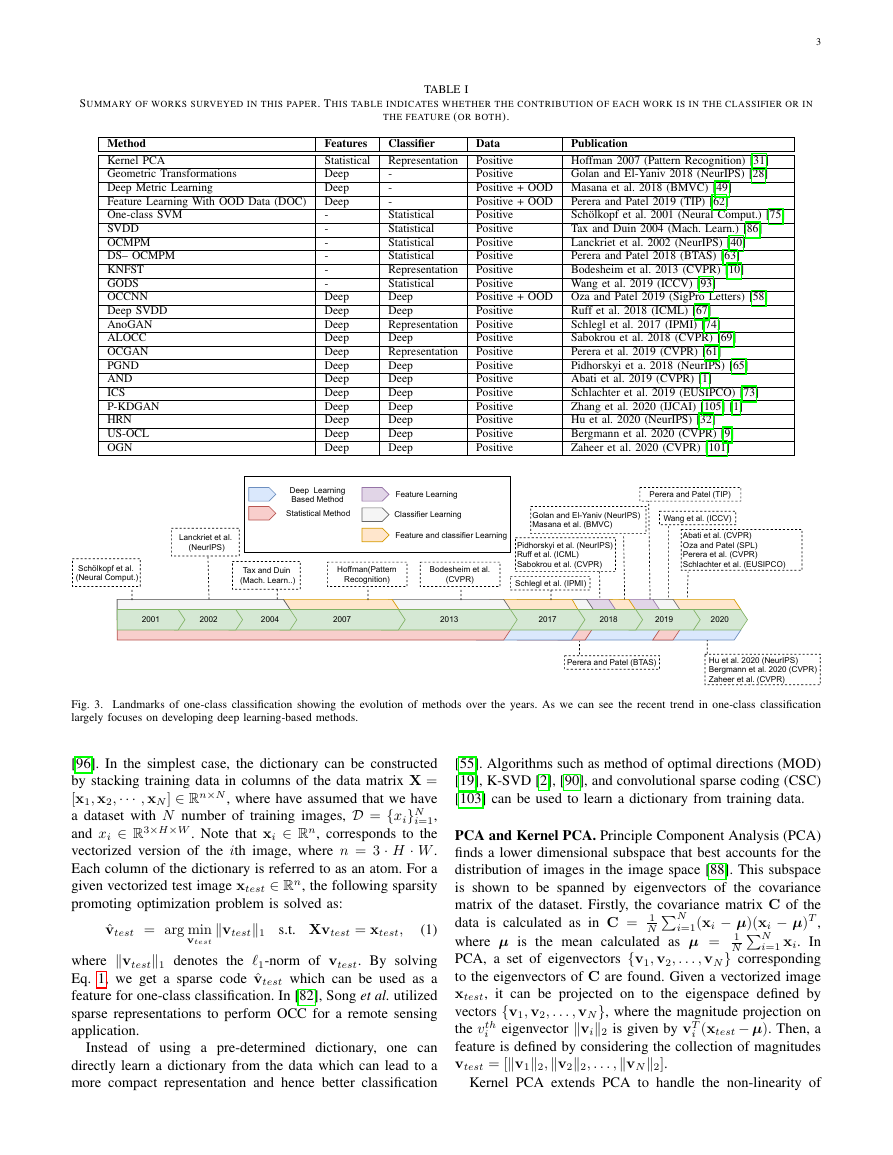In Figure 3, landmarks of OCC are illustrated with a break down of their contributions (feature learning, classiﬁer learning, both feature and classiﬁer learning). We further indicate whether each method is based on a statistical learning 2 framework or a deep learning framework in Figure 3. Initial works on OCC primarily used statistical features and focused on developing classiﬁers. Most methods since 2017 have used deep features in their frameworks. These methods either use classical classiﬁers on deep features or simultaneously learn both features and classiﬁer. In Table II we summarize papers we survey in this work and specify their contributions with respect to the taxonomy we provided. III. FEATURES FOR OCC Learning features that aid in classiﬁcation is a well re- searched problem in multi-class classiﬁcation. In order to perform classiﬁcation correctly, a suitable feature should be selected such that a classiﬁer can deﬁne regions where objects from each class appear consistently. Similar to multi-class classiﬁcation, OCC will beneﬁt from features that position data of the positive class separately from the other objects in the world. However, learning/selecting such a feature is a more difﬁcult task as there are no non-positive data available during training. Nevertheless, following two properties can be identiﬁed in a desired feature for one class classiﬁcation [62]: 1) Compactness. A desired quality of a feature is to have a similar feature representation for different images of the same class. Hence, a collection of features extracted from a set of images of a given class will be compactly placed in the feature space. 2) Descriptiveness. The given feature should produce dis- tinct representations for images of different classes. Ide- ally, each class will have a distinct feature representation from each other. Earliest of features in computer vision were engineered manually with the objective of providing good description of the image [17], [3], [46]. These features are known as hand-crafted features. Later, researchers used data-driven ap- proaches to discover more discriminative features through optimization. In [91], intra-class distance was minimized while maximizing inter-class distance to learn an informative feature embedding. It was later shown by [96] that sparse representa- tion based on a dictionary can lead to better discriminative features. More recent works on feature learning use deep- learning with cross-entropy loss and triplet similarity loss to learn features for multi-class classiﬁcation. Traditional hand-crafted features [17], [3] can be used for OCC as well. Use of hand crafted features are not any different from multiple-class classiﬁcation in this case. On the other hand, data-driven feature learning methods such as LDA [91] and deep-feature learning do not ﬁt well in OCC framework due to the absence of multiple classes. However, data-driven methods that do not use class label information for feature learning such as PCA [88], KPCA [77] and sparse coding can be used for one class feature learning. Usage of these data- driven methods for one class feature extraction is not different from the methodology used in multi-class classiﬁcation. A. Statistical Features Sparse Coding. Given a query image, sparse representation- based methods extract features with respect to a dictionary

3 SUMMARY OF WORKS SURVEYED IN THIS PAPER. THIS TABLE INDICATES WHETHER THE CONTRIBUTION OF EACH WORK IS IN THE CLASSIFIER OR IN TABLE I THE FEATURE (OR BOTH). Method Kernel PCA Geometric Transformations Deep Metric Learning Feature Learning With OOD Data (DOC) One-class SVM SVDD OCMPM DS– OCMPM KNFST GODS OCCNN Deep SVDD AnoGAN ALOCC OCGAN PGND AND ICS P-KDGAN HRN US-OCL OGN Features Statistical Deep Deep Deep - - - - - - Deep Deep Deep Deep Deep Deep Deep Deep Deep Deep Deep Deep Classiﬁer Representation - - - Statistical Statistical Statistical Statistical Representation Statistical Deep Deep Representation Deep Representation Deep Deep Deep Deep Deep Deep Deep Publication Hoffman 2007 (Pattern Recognition) [31] Golan and El-Yaniv 2018 (NeurIPS) [28] Data Positive Positive Positive + OOD Masana et al. 2018 (BMVC) [49] Perera and Patel 2019 (TIP) [62] Positive + OOD Sch¨olkopf et al. 2001 (Neural Comput.) [75] Positive Tax and Duin 2004 (Mach. Learn.) [86] Positive Lanckriet et al. 2002 (NeurIPS) [40] Positive Perera and Patel 2018 (BTAS) [63] Positive Positive Bodesheim et al. 2013 (CVPR) [10] Wang et al. 2019 (ICCV) [93] Positive Oza and Patel 2019 (SigPro Letters) [58] Positive + OOD Ruff et al. 2018 (ICML) [67] Positive Schlegl et al. 2017 (IPMI) [74] Positive Positive Sabokrou et al. 2018 (CVPR) [69] Perera et al. 2019 (CVPR) [61] Positive Pidhorskyi et a. 2018 (NeurIPS) [65] Positive Abati et al. 2019 (CVPR) [1] Positive Schlachter et al. 2019 (EUSIPCO) [73] Positive Positive Zhang et al. 2020 (IJCAI) [105] [1] Hu et al. 2020 (NeurIPS) [32] Positive Bergmann et al. 2020 (CVPR) [9] Positive Positive Zaheer et al. 2020 (CVPR) [101] Fig. 3. Landmarks of one-class classiﬁcation showing the evolution of methods over the years. As we can see the recent trend in one-class classiﬁcation largely focuses on developing deep learning-based methods. [96]. In the simplest case, the dictionary can be constructed by stacking training data in columns of the data matrix X = [x1, x2,··· , xN ] ∈ Rn×N , where have assumed that we have a dataset with N number of training images, D = {xi}N i=1, and xi ∈ R3×H×W . Note that xi ∈ Rn, corresponds to the vectorized version of the ith image, where n = 3 · H · W . Each column of the dictionary is referred to as an atom. For a given vectorized test image xtest ∈ Rn, the following sparsity promoting optimization problem is solved as: vtest1 s.t. Xvtest = xtest, ˆvtest = arg min vtest (1) where vtest1 denotes the 1-norm of vtest. By solving Eq. 1, we get a sparse code ˆvtest which can be used as a feature for one-class classiﬁcation. In [82], Song et al. utilized sparse representations to perform OCC for a remote sensing application. Instead of using a pre-determined dictionary, one can directly learn a dictionary from the data which can lead to a more compact representation and hence better classiﬁcation [55]. Algorithms such as method of optimal directions (MOD) [19], K-SVD [2], [90], and convolutional sparse coding (CSC) [103] can be used to learn a dictionary from training data. PCA and Kernel PCA. Principle Component Analysis (PCA) ﬁnds a lower dimensional subspace that best accounts for the distribution of images in the image space [88]. This subspace N is shown to be spanned by eigenvectors of the covariance matrix of the dataset. Firstly, the covariance matrix C of the i=1(xi − µ)(xi − µ)T , data is calculated as in C = 1 N where µ is the mean calculated as µ = 1 i=1 xi. In PCA, a set of eigenvectors {v1, v2, . . . , vN} corresponding N to the eigenvectors of C are found. Given a vectorized image xtest, it can be projected on to the eigenspace deﬁned by vectors {v1, v2, . . . , vN}, where the magnitude projection on i (xtest − µ). Then, a the vth i feature is deﬁned by considering the collection of magnitudes vtest = [v12,v22, . . . ,vN2]. eigenvector vi2 is given by vT N Kernel PCA extends PCA to handle the non-linearity of 2020Deep LearningBased MethodStatistical MethodFeature LearningAbati et al. (CVPR)Oza and Patel (SPL)Perera et al. (CVPR) Schlachter et al. (EUSIPCO)Perera and Patel (TIP)Classifier LearningFeature and classifier Learning 2019Golan and El-Yaniv (NeurIPS)Masana et al. (BMVC)Pidhorskyi et al. (NeurIPS)Ruff et al. (ICML)Sabokrou et al. (CVPR)Perera and Patel (BTAS)Schlegl et al. (IPMI)201820172013Bodesheim et al.(CVPR)2007Hoffman(PatternRecognition)Schölkopf et al. (Neural Comput.)200220012004Lanckriet et al. (NeurIPS)Tax and Duin (Mach. Learn..)Wang et al. (ICCV) Hu et al. 2020 (NeurIPS) Bergmann et al. 2020 (CVPR) Zaheer et al. (CVPR)

data [77]. Let us assume that we have a mapping function Φ : Rn → Rd that can map data xi into a feature space Φ(xi). Depending on the mapping function, the feature space dimension d can be arbitrarily large. For simplicity let us assume the data mapped into the feature space is centered, i=1 Φ(xi) = 0. As a result, the covariance matrix in i.e., 1 N the feature space can be computed as follows: N Φ(xi)Φ(xi)T , (2) N i=1 ¯C = 1 N i=1 αj i Φ(xi), where αj as vj = N To perform PCA in the feature space, we need to ﬁnd a set of eigenvectors and non-zero eigenvalues in the feature space. Let λj and vj denote the eigen values and the corresponding eigen vector of ¯C, respectively. One can represent eigen vectors N are a set of coefﬁcients. Since the eigenvalue and eigenvectors must satisfy λjvj = ¯Cvj, for performing PCA in the feature space, we consider an equivalent system as: λjΦ(xi), vj = Φ(xi), ¯Cvj, λjΦ(xi), for i = 1, . . . , N, i Φ(xl), αj i Φ(xl) = Φ(xi), ¯C αj N 1, αj 2, . . . , αj N (3) (4) l=1 l=1 where, ·,· indicates inner product between two vectors. Let us deﬁne a column vector as αj = [αj N ]T and a non-singular N × N matrix K, where each entry of the matrix is deﬁned as, Krt := Φ(xr), Φ(xt). Using these notations, we can simplify the above equation as: 2, . . . , αj 1, αj N λjαj = Kαj. (5) Then the solution αj belonging to non-zero eigenvalues is found by requiring that corresponding vectors in Rd be normalized, i.e., vj, vj = 1 [95]. Consequently, we can ﬁnd the corresponding eigenvectors vj. For a new vectorized test image xtest, we can compute its projection onto the eigenvectors. We can calculate the projection with respect to the jth eigenvector in the feature space as: vj, Φ(xtest) = iΦ(xi), Φ(xtest). αj (6) i=1 Note that in Eq. 6, we do not require the deﬁnition of mapping function Φ in its explicit form and only need it in the dot product form. Hence, we can deﬁne functions to perform dot products without actually having to explicitly map data points using the mapping function Φ. These functions are commonly referred to as kernel functions [30]. An example of a kernel function is the the RBF kernel [30], deﬁned as K(xi, xj) = e−xi−xj2/2σ2 , where σ is a parameter of the kernel. Similar to PCA, the projection values computed using Eq. 6 are used as a feature representation for any test data. Note that, kernel PCA can be derived for data without the assumption that data is centered in feature space with minor modiﬁcation in the derivation process [76]. Both PCA and kernel PCA produce features that are de- scriptive as the lower dimensional subspace learned has the capacity to represent the image space of training data [31]. However, the learned embeddings are not necessarily compact. 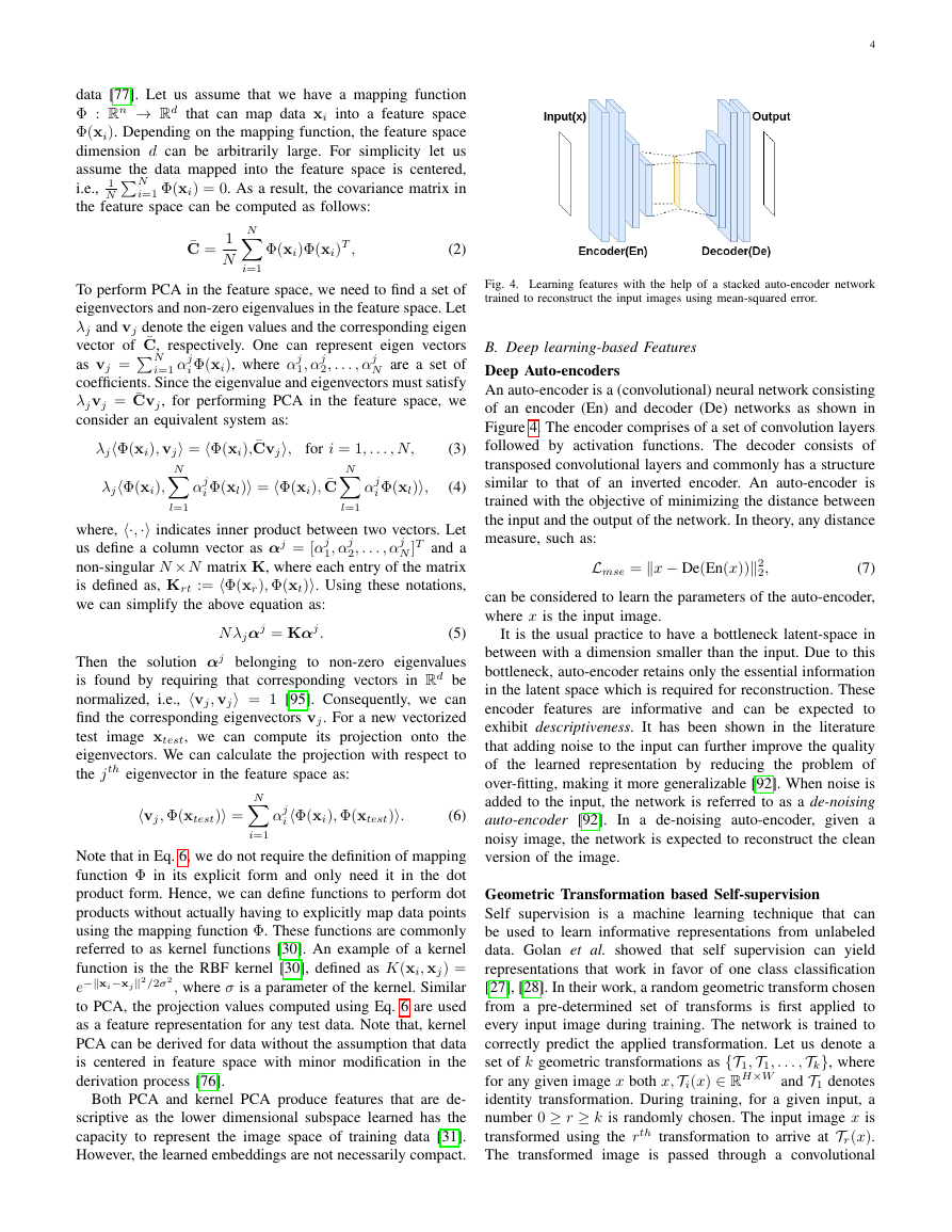N 4 Fig. 4. Learning features with the help of a stacked auto-encoder network trained to reconstruct the input images using mean-squared error. B. Deep learning-based Features Deep Auto-encoders An auto-encoder is a (convolutional) neural network consisting of an encoder (En) and decoder (De) networks as shown in Figure 4. The encoder comprises of a set of convolution layers followed by activation functions. The decoder consists of transposed convolutional layers and commonly has a structure similar to that of an inverted encoder. An auto-encoder is trained with the objective of minimizing the distance between the input and the output of the network. In theory, any distance measure, such as: Lmse = x − De(En(x))2 2, (7) can be considered to learn the parameters of the auto-encoder, where x is the input image. It is the usual practice to have a bottleneck latent-space in between with a dimension smaller than the input. Due to this bottleneck, auto-encoder retains only the essential information in the latent space which is required for reconstruction. These encoder features are informative and can be expected to exhibit descriptiveness. It has been shown in the literature that adding noise to the input can further improve the quality of the learned representation by reducing the problem of over-ﬁtting, making it more generalizable [92]. When noise is added to the input, the network is referred to as a de-noising auto-encoder [92]. In a de-noising auto-encoder, given a noisy image, the network is expected to reconstruct the clean version of the image. Geometric Transformation based Self-supervision Self supervision is a machine learning technique that can be used to learn informative representations from unlabeled data. Golan et al. showed that self supervision can yield representations that work in favor of one class classiﬁcation [27], [28]. In their work, a random geometric transform chosen from a pre-determined set of transforms is ﬁrst applied to every input image during training. The network is trained to correctly predict the applied transformation. Let us denote a set of k geometric transformations as {T1,T1, . . . ,Tk}, where for any given image x both x,Ti(x) ∈ RH×W and T1 denotes identity transformation. During training, for a given input, a number 0 ≥ r ≥ k is randomly chosen. The input image x is transformed using the rth transformation to arrive at Tr(x). The transformed image is passed through a convolutional

neural network and the network parameters are optimized with a cross-entropy loss where r is considered to be the ground truth label. The trained network produces features suitable for one class classiﬁcation. Golan et al. [28] showed that a neural network trained in this manner produces relatively higher probability scores in the ground truth class for samples of the positive class. For a given test image xtest, [28] proposed to evaluate a normality score stest by considering log likelihood probability of the ground truth class with all k transformations as: stest(xtest) = log(F (Ti(xtest))), (8) where F (·) is the softmax output of the network. Further- more, Golan et al. [28] derived a Dirichlet distribution-based score which is more effective for one class classiﬁcation. This second score was derived by assuming that each con- ditional distribution takes the form of a Dirichlet distribution F (Ti(x))|Ti ∼ Dir(ai) where ai ∈ Rk +. When estimates of Dirichlet parameters ˆai are found with the help of maximum likelihood estimation, the ﬁnal normality score denoted as utest can be expressed as: utest(xtest) = (ˆai − 1) · f (Ti(x)), (9) k i=1 k i=1 it Deep Metric Learning with OOD Data A contrastive loss-based metric learning method is proposed in [49] to learn features for OCC. For the metric learning process, [49] proposes to use data from an OOD dataset. In the absence of an OOD dataset, is artiﬁcially generated by adding random Gaussian noise to the images. Let F be the network function of a deep convolutional network. For a pair of input images x1 and x1, the distance between the to inputs in the feature space is deﬁned as K(x1, x2) = F (x1) − F (x2)2. The training process incorporates two types of labels. Label γ indicates whether the two inputs belong to the same class (γ = 0) or not (γ = 1). Label ζ denotes if both images belong to a OOD dataset (ζ = 0) or not (ζ = 1). The contrastive loss is deﬁned as: L = 1 2 (1 − γ) · ζ · K(x1, x2)2 2 γ · ζ · (max(0, m − K(x1, x2))2, + 1 (10) where, m denotes minimum margin. For positively labeled data when both images are from the same class (γ = 0, ζ = 1), the loss becomes 1 2 K(x1, x2)2. Therefore, during training network learns a similar embedding for positive data. As a result, the compactness property is satisﬁed. On the other hand, when the image pair is from different classes, the embedding is encouraged to be at least m distance apart in the feature space. In the case when both images are from the same class (γ = 0, ζ = 0), the loss becomes zero. Therefore, the learned feature embedding becomes descriptive with the ability of differentiating positively labeled and data outside the given category. Feature Learning With OOD Data (DOC) In [62], authors consider the special scenario where a set of 5 labeled Out Of Distribution (OOD) data is available during training along side positive data. These OOD data are data collected from non-overlapping problem domain. For exam- ple, in the case of a face recognition problem for one-class classiﬁcation an annotated object dataset can be considered as OOD. This setting is important in practice as many real life applications of OCC can be solved in this setting. Let us consider a deep network with a feature extraction sub-network F and a classiﬁcation sub-network G. The network G ◦ F is ﬁrst trained using the OOD data using cross entropy loss. Let us denote the positively labeled dataset with N number of training images as Dt = {xti}N i=1 and OOD dataset with M number of images as Dr = {xri, yri}M i=1, where images xti, xri ∈ R3×H×W and yri is the target label for the image xri. The features extracted from any image xti are denoted as F (xti) = zti ∈ Rd. Here, d is the dimension of the feature space. A compactness loss Lc is deﬁned that measures compactness of the learned feature with respect to positive data. The compactness loss is evaluated using a intra-class distance for that given batch in the feature space as: 1 d Lc(xti) = (zti − µti)T (zti − µti), (11) where feature extracted from each image xti zti ∈ Rd. The mean vector µti j=i ztj. Additionally, a descriptiveness loss denoted as Ld is used to measure descriptiveness of the learned features. It is measured using cross-entropy loss obtained by the output of the network with respect to OOD data. The network is ﬁne-tuned by jointly optimizing over both compactness and descriptiveness loss as: is deﬁned as µti = 1 N−1 Ld(xri, yri) + λ Lc(xti), (12) i=1 i=1 where, xri and xti denote data from the OOD dataset and the positively labeled data respectively and λ is a hyper-parameter. As a result, the learned feature is both descriptive and compact with respect to the positively labeled data. IV. OCC ALGORITHMS A. Representation-based Methods In Section. III-A, we discussed statistical methods that can be used to obtain features for one class classiﬁcation. These methods encode information present in the input image to a feature vector. Once the feature corresponding to any query image is obtained, it can be used to perform classiﬁcation using two different strategies. In the ﬁrst strategy, the feature is mapped back to the image space to obtain a reconstructed image. Then, reconstruction error is calculated in the image space. In the second strategy, the feature representation is used to calculate a distance measure which can encode the score of query image with respect to training data. The sparse coding and PCA falls into the former strategy. On the other hand, kernel based one class classiﬁcation utilizes the latter strategy. The detailed discussion on sparse coding and PCA/Kernel PCA based one-class methods is provided in Section. III-A. Here, we focus on another method that obtains a score measure for any query image using Foley-Sammon M min F,G N

Transform (FST) to learn a “null space” of the training data. Kernel Null Foley–Sammon Transform (KNFST) FST or Fisher transform is commonly used for linear dis- criminant analysis in the ﬁeld of subspace methods [23]. Null Foley–Sammon Transform (NFST) [10] is a special case of FST or Fisher transform, which is used to learn transformation from multi-class data. The goal of NFST is to learn a mapping w, where intra-class distances are zero while inter-class distances remain positive by solving the following equations for ϕ: wT Cww = 0, wT Cbw > 0, (13) (14) where, Cb and Cw are the inter-class/between-class and intra-class/within-class covariance/scatter matrix, respectively. When the sample size is small n ≤ d, there exists k − 1 null projection directions w(1), . . . , w(k−1), for a k class problem. When the total scatter is deﬁned as Ct = Cb + Cw and when wT Cww = 0 holds, the objective boils down to ﬁnding w with wT Cbw > 0. It was shown in [10] that these two conditions are satisﬁed t ∩ Zw) where Zw is the null when w(1), . . . , w(k−1) ∈ (Z⊥ N space of Cw and Z⊥ is the row space of Ct. We can show that t can be exactly spanned with x1−µ, . . . , xN −µ with µ = Z⊥ i=1 xN . Therefore, to ensure w ∈ Z⊥ t we can represent 1 N each w with weighted combination of some orthonormal basis {b1, . . . , bn} as: t w = β1b1 + ··· + βnbn, (15) where, βi are scalar coefﬁcients, bi ∈ Rn and n ≤ N. The basis {bi}n i=1 can be obtain through Gram-Schmidt orthonormalization or principle component analysis. Let us denote a vector β = [β1, . . . , βn] and B = [b1, . . . , bn]T . Hence, we can denote mapping w = Bβ. By substituting in Eq. 13, we get βT (BT CwB)β = 0. Solution to this equation can be found by solving the following eigenvalue problem: (BT CwB)β = 0. (16) Solution vectors β can be used to calculate Q. Since the ˜X ˜XT , where scatter matrix Cw is expressed as Cw = 1 ˜X is obtained by stacking zero-mean data vectors {x1 − N µ, . . . , xN − µ} as columns, Eq. 16 can be re-written as: (BT ˜X ˜XT B)β = 0. (17) Since all terms in Eq. 17 appear as product terms, a kernelized version of the problem can be obtained by replacing product terms with a kernel functions K(·,·) following similar steps as discussed in Section III-A about kernel PCA. Mapping data to a higher dimensional space through kernelization relaxes the condition that the dataset size should be small sample size is small n ≤ N. When formulating Null Foley–Sammon Transform in the one-class setting, the origin of the coordinate space is treated as the negative class similar to one-class SVM. Then, a single null-space vector w is learned considering positive data. First, mean removed training data ˜X, is projected by the null-space 6 vector w to obtain vector t. During inference, a mean removed query image xtest−µ is projected using w to obtain t∗. When the difference |t−t∗| is lower than a pre-determined threshold, the query is assigned with a positive class identity. B. Statistical Methods One Class Support Vector Machine (OCSVM) One class SVM is a special case of Support Vector Machine (SVM) formulation. In a binary SVM, the hyper-plane that separates the two classes with that largest possible margin is found. The hyper-plane is deﬁned by support vectors. In the case of one class classiﬁcation, there exists only positively labeled data during training. In One Class SVM (OCSVM), hyperplane corresponding to negative class are set to be the origin of the coordinate system [75]. Therefore, the objective of OCSVM boils down to ﬁnding a hyper-plane furthest away from the origin, where positively labeled data exists in the positive half space of the hyper-plane. When this constraint is relaxed using slack variables, the optimization objective can be written as: i ξi − b w, Φ(xi) ≥ b − ξi, ξi ≥ 0, 2||w||2 + 1 νN 1 min w,ξ,b s.t. (18) Eq. 18 can be modiﬁed with the help of Lagrange multipli- where, the column vector ξ = [ξi, ξ2, . . . , ξN ] and each ξi is the slack variable corresponding to the ith training sample (i.e. vectorized image), Φ is a mapping function that maps xi to a kernel space where dot products are deﬁned using a kernel function K(·,·), b is the bias term and ν is a trade-off parameter, and N is number of training examples. When the optimization is solved, inference on a query sample xtest can be done using the condition sgn(w, φ(x) − b). ers αi, βi ≥ 0 as follows: L(w, ξ, b, α, β) = 1 2 αi(w, Φ(xi) − b + ξi) − variables to zero, it can be shown that w = − where the column vectors α = [αi, α2, . . . , αN ]T and β = [βi, β2, . . . , βN ]T . Setting derivatives with respect to primal iαi, Φ(xi), i αi = 1. By substituting these αi = 1 values in Eq. 18, the dual optimization problem can be derived as: νN and νN − βi ≤ 1 ||w||2 + ξi − b 1 νN βiξi, (19) i i i min α s.t. 1 2 i 0 ≤ αi ≤ 1 j αiαjK(xi, xj) i αi = 1. (20) νN , Furthermore, it can be shown that when 0 ≤ αi ≤ 1 satisﬁed the bias term can also be expressed as: νN is b = w, Φ(xi) = αjK(xi, xj). (21) j With the dual form of the problem, as shown in Eq. 20, the optimal values of parameters in problem shown in Eq. 18 can be found using the kernel function K(·,·) without explicitly deﬁning the mapping function Φ(·). The decision for any test image xtest that is vectorized as xtest can also be expressed

in terms of the kernel function using the dual variables and vectorized training images as follows: sgn( αiK(xi, xtest) − b), (22) i Support Vector Data Descriptor (SVDD) The SVDD [86] formulation closely follows the OCSVM ob- jective. However, instead of learning a hyper-plane to separate data from origin, Tax et al. [86] propose to ﬁnd the smallest hyper-sphere that can ﬁt given training samples. The hyper- sphere is characterized by its mean vector (or centroid of hyper-sphere) o and radii rd > 0. The volume of hyper-sphere is minimized by minimizing rd ∈ R while making sure hyper- sphere encloses most of the training samples. This objective can be written down in the form of optimization problem as: min o,ξ,rd s.t. xi − o2 ≤ r2 d + ξi, ξi ≥ 0 ∀i. (23) Parameter λ controls the trade-off between errors and the objective. Similar to the OCSVM, the above objective can be modiﬁed with the help of the Lagrangian multipliers and the updated optimization problem can be re-formulated as: d + ξi− L(rd, o, α, γ, ξ) = r2 ξi − αi(r2 d + λ (xi2 − 2o, xi + o2)) − i αi = 1, o = to zero, it can be shown that where, the column vectors α = [αi, α2, . . . , αN ]T and γ = [γi, γ2, . . . , γN ]T . By setting derivatives of primal variables i αixi and λ− αi− γi = 0. By substituting to Equation 24, the dual form can be obtained as: i i i d + λ r2 i ξi i min α j αiαjxi, xj − s.t. 0 ≤ αi ≤ λ, xtest − o2 = xtest, x − 2 αix, xi αiαjxi, xj ≤ r2 d. i + A given test sample xtest, is assigned a positive label if it is inside the identiﬁed hyper-sphere. More precisely, if the following condition is met: i αixi, xi i αi = 1. (25) 7 becomes constant and the optimization becomes equivalent to the dual form of OCSVM in Equation 20 discussed in the previous section. One Class Mini-max Probability Machine (OCMPM) Similar to in one-class SVM, One class Mini-max Probability Machine (1-MPM) tries to maximize the distance between the origin and learned hyper-place with the objective of arriving at a tighter lower bound to the data. However, 1-MPM takes advantage of second order statistics of training data when the hyper-plane is learned. In the 1-MPM algorithm, both N mean µ and the covariance matrix C of the vectorized images is calculated. The covariance matrix can be calculated as i=1(xi − µ)(xi − µ)T , where µ is the mean is C = 1 N i=1 xN . Furthermore, 1-MPM does not calculated as µ = 1 N assume any distribution of the underlying data x unlike PCA (which has inherent assumption of data belonging to Gaussian distribution). With the help of both mean and covariance information of the data, 1-MPM seeks to ﬁnd a hyper-plane (w, b) with w ∈ Rn \ {0}, b ∈ R such that data lies in the positive half space deﬁned by {x|x ∈ Rn, wT x ≥ b}, at least with a probability of τ, even in the worst case scenario. With this background, the objective function of single class MPM can be formulated as in: N (24) γiξi, max w=0,b b√ wT Cw s.t. inf (x,µ,C) P (wT x ≥ b) ≥ τ, (28) when the distance between the origin and the hyper-plane is measured in terms of Mahalonabis distance with respect to C. Since this problem is positively homogeneous in (w, b) and because w = 0 is always satisﬁed when b > 0, value of b is taken to be one without loss of generality. Then, a equivalent optimization problem can be obtained by minimizing the reciprocal of Mahalonobis distance as in: min w wT Cw s.t. inf (x,µ,C) P (wT x ≥ 1) ≥ τ, (29) Using the core MPM theorem in [39], where it is stated that inf (x,µ,C) P (wT x ≥ b) ≥ τ is equivalent to b− wT ˆx ≥ √ 1−τ , Equation 29 can be re- g(τ ) written as: wT C, where g(τ ) = τ √ (26) min w wT C 1 22 s.t. 1 − wT µ ≥ g(τ )wT C 1 22. (30) i j Since, the dual form and the inference equation both include inner product terms of xi and x, SVDD can be extended to a kernel formulation by simply replacing product terms by a kernel function that corresponds to some mapping function Φ as, Φ(xj), Φ(xi) = K(xi, xj). The kernalized version of the optimization problem of dual form then can be expressed as: j αiαj(K(xi, xj) − As we mentioned earlier that 0 ≤ αi ≤ C, i αi = 1. Due to that in the case where the kernel function only depends on the difference between the two vectors, i.e., when K(x1, x2) depends only on x1 − x2, the linear term of the dual objective function i αi(K(xi, xi))) i αi = 1. (27) min s.t. α i Here it should be noted that for a real symmetric covariance matrix C, the matrix C 1 2 always exists. Since optimization problem shown in Equation 30 is a second order cone program it can be efﬁciently solved using convex optimization tools. it In the robust 1-MPM formulation, is assumed that difference between sample covariance and true covariance of the distribution will not exceed some arbitrary constant denoted as ρ and Mahalanobis distance between sample mean and true mean with respect to true covariance will not exceed an arbitrary constant denoted as ν2 [39]. Under these assumptions, it is shown in [40] that wT Cw term in Equation 29 gets substituted by wT (C + ρIn)w, while g(τ ) term is changed into K(τ ) + ν. Dual slope Mini-max Probability Machine (DS–OCMPM)

Dual slope Mini-max Probability Machine is a an exten- sion of 1-MPM considering two decision hyper-planes and availability of sub-clusters [63]. In [63], a second hyper-plane ( ˜w, ˜b) is learned such that the data projected on the hyper- plane ˜w has the largest possible variance. The optimization objectives takes the form of: √ max ˜w ˜wT C ˜w s.t. inf x,µ,C) P ( ˜wT x ≥ 1) ≥ ˜τ . (31) √ √ Since maximizing ˜wT C ˜w is equivalent to minimizing ˜wT C−1 ˜w. Optimization problem in Equation 31 can be transformed into another second order cone program of the form: ˜wT C− 1 22 s.t. 1 − ˜wT µ ≥ g(˜τ ) ˜wT C− 1 22. (32) min ˜w Assuming that the difference between sample covariance and true covariance of the distribution will not exceed some arbitrary constant ˜ρ for C−1, the robust version of the opti- mization problem is obtained by substituting ˜wT C−1 ˜w term in Equation 31 by ˜wT (C + ˜ρIn) −1 ˜w. In order to mitigate the effect of sub-distributions, data is clustered into k clusters using the Ward’s method [94]. Global mean and variance (µ, C) are calculated with respect to the whole dataset along with cluster-wise statistics (µi, Ci) for ith cluster. Optimization is carried out over cumulative covariance wT Ciw while constraints are of each individual cluster i deﬁned with respect to global statistics (µ, C). Given global and local clusters (µ, C) and (µi, Ci) for i = 1, 2, . . . , k, where k is the number of clusters, the following joint-optimization problem is solved to ﬁnd both w and ˜w: w, ˜w ||wT (Ci + ρIn) minimize subject to (g(˜τ ) + ν)|| ˜wT (Ci + ˜ρIn)− 1 i=1 1 22 2||2 + ˜wT (Ci + ˜ρIn)− 1 2||2 − 1 ≤ ˜wT µ 22 − 1 ≤ wT µ. 1 (g(τ ) + ν)wT (Ci + ρIn) statement, (33) Since the product of w and ˜w do not appear in the optimization be solved independently for w and ˜w using two second order cone programs. Once hyper-plane parameters are obtained, given a test sample xtest, identity of the sample would be assigned to be negative if wT xtest < 1 ∩ ˜wT xtest < 1, and positive otherwise. problem can this k using the following optimization objective: min (w,b),( ˜w,˜b),ξ, ˜ξ,β>0 s.t. 1 −b − ˜b + λ 2||w||2 + ˜w2 i ξi + ˜ξi wT xi − b ≥ η − ξi, ˜wT xi − ˜b ≤ η − ˜ξi, dist((w, b), ( ˜w, ˜b)) ≤ β, 8 (34) (35) where, λ is the slack regularization constant, η deﬁnes the classiﬁer margin and dist(·,·) is suitable distance function between the two hyper-planes. This loss function forces to ﬁnd the most similar pair of hyper-planes that satisﬁes the stated objective. The additional constraint on distances prevents from ﬁnding a trivial solution. By explicitly setting w2 2 = 1 and ˜w2 2 = 1 and setting dist(·,·) to be the Euclidean distance, this objective can be simpliﬁed as: b,˜b,ξ,ξ,β>0 min s.t. g(b, ˜b) − 2 wT ˜w + λ i ξi + ˜ξi iη − (wT (xi + b) − ξi+ +η − ( ˜wT (xi + ˜b) − ˜ξi+, 2 = 1, 2 = 1, ˜w2 w2 where g(b, ˜b) = (b − ˜b)2 − b − ˜b and notation + denotes hinge loss. This initial formulation can be extended to a generalized formulation by introducing sub-spaces in place of hyper-planes. Let W, ˜W ∈ SM n be orthonormal subspace frames, where WT W = ˜WT ˜W = IM . Here, IM is identity matrix of size M × M. Such frames SM n with n dimensional subspaces, belong to the Stiefel manifold and each column in the matrices W, ˜W of size n × M is orthonormal to the rest. The number of hyper-planes M is a hyper-parameter and can be set differently for each dataset to achieve better per- formance. By replacing the distance term dist((w, b), ( ˜w, ˜b)) by the Euclidean distance of each data point from both hyper- N planes, Equation 36 can be modiﬁed as: + g(b, ˜b) + λ i=1(WT xi + b2 iη − min(WT (xi + b) − ξi2 + iη + max( ˜WT (xi + ˜b) − ˜ξi2 +. (36) Classiﬁer obtained by solving this optimization is named as the generalized one-class discriminative subspace (GODS) classiﬁer. [93] presents a parameter initialization method and an efﬁcient optimization method to optimized the proposed optimization objective. 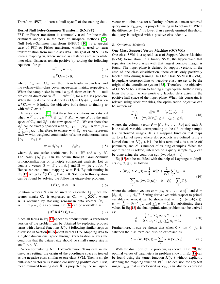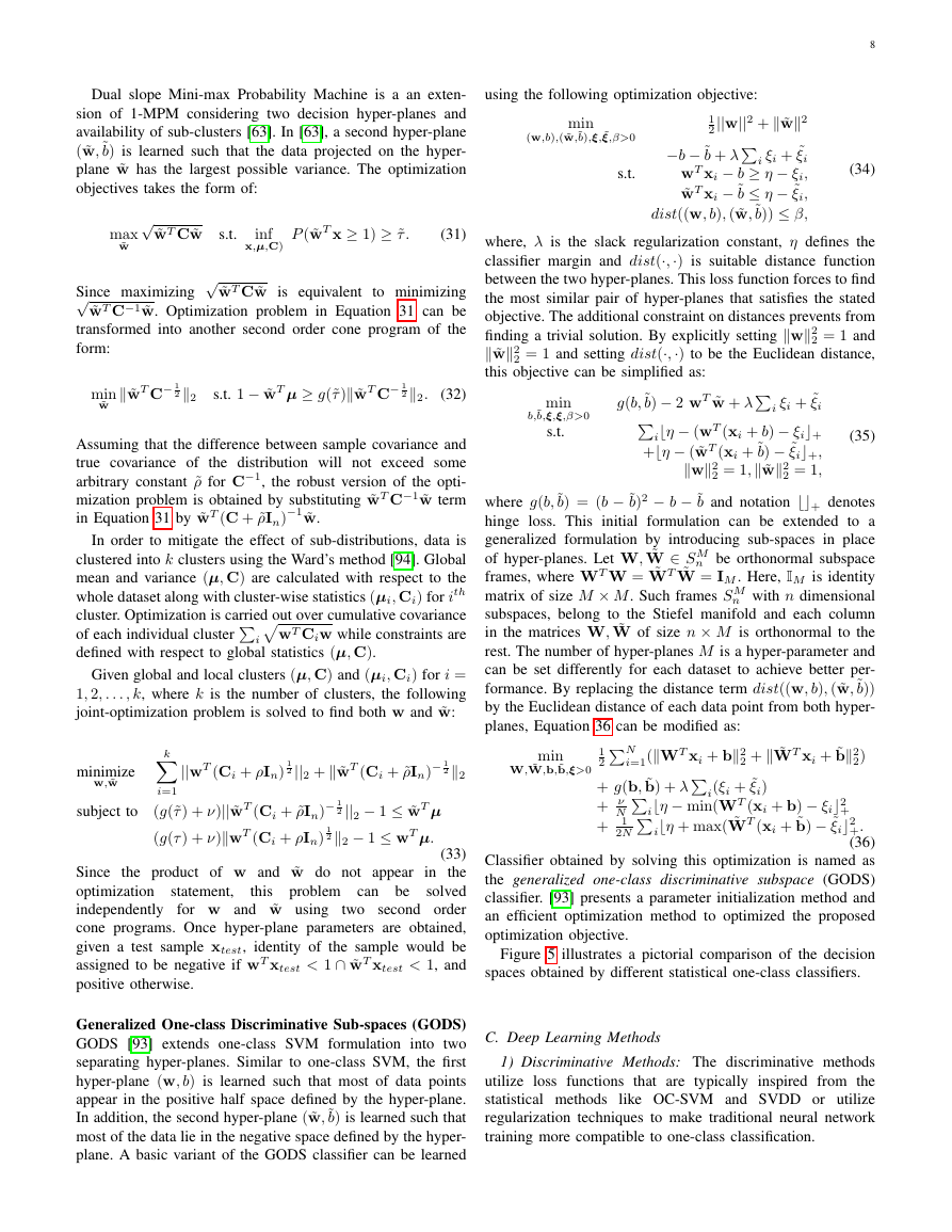2 + ˜WT xi + ˜b2 2) + ν N + 1 2N i(ξi + ˜ξi) W, ˜W,b,˜b,ξ>0 min 1 2 Figure 5 illustrates a pictorial comparison of the decision spaces obtained by different statistical one-class classiﬁers. Generalized One-class Discriminative Sub-spaces (GODS) GODS [93] extends one-class SVM formulation into two separating hyper-planes. Similar to one-class SVM, the ﬁrst hyper-plane (w, b) is learned such that most of data points appear in the positive half space deﬁned by the hyper-plane. In addition, the second hyper-plane ( ˜w, ˜b) is learned such that most of the data lie in the negative space deﬁned by the hyper- plane. A basic variant of the GODS classiﬁer can be learned C. Deep Learning Methods 1) Discriminative Methods: The discriminative methods utilize loss functions that are typically inspired from the statistical methods like OC-SVM and SVDD or utilize regularization techniques to make traditional neural network training more compatible to one-class classiﬁcation.

分享到：

赞收藏

资料库

20年单类别(One-Class)分类全面综述论文.pdf

相关推荐

人工智能

热门标签

最新资料