Creating SCS Curve Number Grid using HEC-GeoHMS
Prepared by
Venkatesh Merwade
School of Civil Engineering, Purdue University
vmerwade@purdue.edu
October 2010
Introduction
SCS curve number grid is used by many hydrologic models to extract the curve number for
watersheds. The objective of this tutorial is to use soil and land use data to create a curve number
grid using HEC-GeoHMS (ArcGIS 9.2 version).
Computer Requirements
You must have a computer with latest windows operating system, and the following programs
installed:
1. ArcGIS 9.3 (with ArcInfo)
2. Arc Hydro tools (latest version)
3. Hec-GeoHMS for ArcGIS 9.3 (latest version)
Make sure the Arc Hydro tools (version that works with 9.2) are installed on the system. There
are lots of Arc Hydro tools available on the internet. The version that is used in this tutorial
including installation instructions is available at the following link.
ftp://ftp.ecn.purdue.edu/vmerwade/download/data/tools.zip
The HEC-GeoHMS set-up file for this tutorial is also included in this above tools.zip file. Just
unzip the file, and run the setup to install both ArcHydro and HEC-GeoHMS. You will need to
have administrative access to install Arc Hydro and HEC-GeoHMS.
Data Requirements and Description
This tutorial requires the following datasets:
(1) DEM for the study area
(2) SSURGO soil data
(3) 2001 land cover grid from USGS
The DEM and land cover grid from USGS and SSURGO data for Cedar Creek in northeast
Indiana are provided as zip file at the end of this paragraph. The SSURGO soil data that will be
used is provided in a geodatabase (cedar_ssurgo.mdb) that is created in the “Downloading
SSURGO Soil Data” tutorial available at:
(http://web.ics.purdue.edu/~vmerwade/education/download_ssurgo.pdf). You can look at the
SSURGO download tutorial if you want to learn how this dataset is processed. Also, if you are
1
�
interested in downloading the DEM and land cover data by yourself, instructions are available in
the following tutorial: http://web.ics.purdue.edu/~vmerwade/education/ned_nhd.pdf
It is highly recommended that you go through these exercises of downloading the data to make
yourself aware of the procedure involved.
(Notes:
1. The DEM, land use and soil data used in this tutorial are already clipped to the Cedar Creek
study watershed
2. This tutorial uses the SSURGO soil data, which is the highest resolution soil data available in
public domain from NRCS. This can be replaced by STATSGO data as long as you know
how to interpret STATSTO to follow the steps provided in this tutorial)
Download the data from ftp://ftp.ecn.purdue.edu/vmerwade/download/data/cngrid.zip
Unzip cngrid.zip in your working directory. The ArcCatalog-view of the data folder (or
whatever name you gave to your working folder) is shown below:
cedar_ssurgo is the geodatabase with SSURGO spatial and tabular data for cedar creek area.
cedar_dem is the raw 30 DEM for Cedar Creek obtained from USGS and clipped for the study
watershed, and cedar_lu is the 2001 land cover grid from USGS. All datasets have a common
spatial reference (NAD_1983_UTM_16).
Note: It is very critical to assign and use consistent coordinate system for all the datasets.
Getting Started
Open ArcMap. Create a new empty map, and save it as cngrid.mxd (or any other name). Right
click on the menu bar to pop up the context menu showing available tools as shown below.
2
�
Check the Arc Hydro Tools 9 menu. If the Arc Hydro Tools menu does not appear in the list,
click on Customize (Scroll down the list to see “Customize”). In the Customize dialog that
appears, check the Arc Hydro Tools box.
You should now see the Arc Hydro tools added to ArcMap as shown below. You can leave it
floating or you may dock it in ArcMap menubars.
Similarly add Spatial Analyst extension and activate it by clicking on ToolsExtensions…, and
checking the box next to Spatial Analyst.
Dataset Setup
All raster data created with the Arc Hydro are stored in a subdirectory with the same name as the
dataset or Data Frame in the ArcMap document (called Layers by default and under the directory
where the project is stored). The location of the vector, raster, and time series data can be
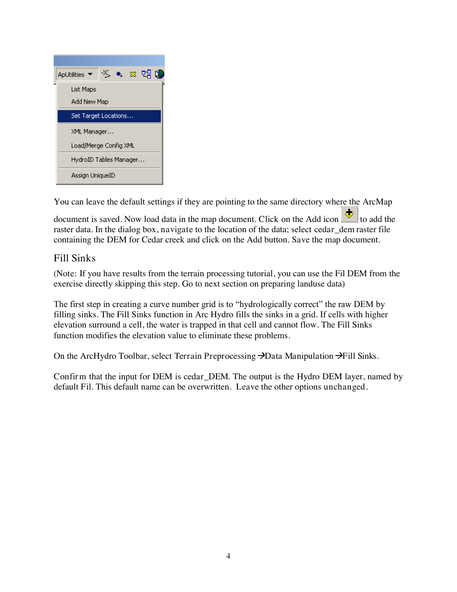
explicitly specified using the function ApUtilitiesSet Target Locations.
3
�
You can leave the default settings if they are pointing to the same directory where the ArcMap
document is saved. Now load data in the map document. Click on the Add icon
raster data. In the dialog box, navigate to the location of the data; select cedar_dem raster file
containing the DEM for Cedar creek and click on the Add button. Save the map document.
to add the
Fill Sinks
(Note: If you have results from the terrain processing tutorial, you can use the Fil DEM from the
exercise directly skipping this step. Go to next section on preparing landuse data)
The first step in creating a curve number grid is to “hydrologically correct” the raw DEM by
filling sinks. The Fill Sinks function in Arc Hydro fills the sinks in a grid. If cells with higher
elevation surround a cell, the water is trapped in that cell and cannot flow. The Fill Sinks
function modifies the elevation value to eliminate these problems.
On the ArcHydro Toolbar, select Terrain PreprocessingData ManipulationFill Sinks.
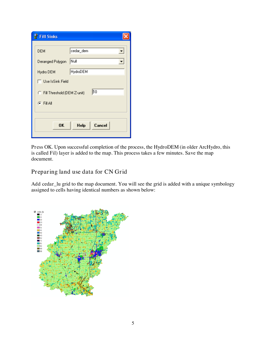
Confirm that the input for DEM is cedar_DEM. The output is the Hydro DEM layer, named by
default Fil. This default name can be overwritten. Leave the other options unchanged.
4
�
Press OK. Upon successful completion of the process, the HydroDEM (in older ArcHydro, this
is called Fil) layer is added to the map. This process takes a few minutes. Save the map
document.
Preparing land use data for CN Grid
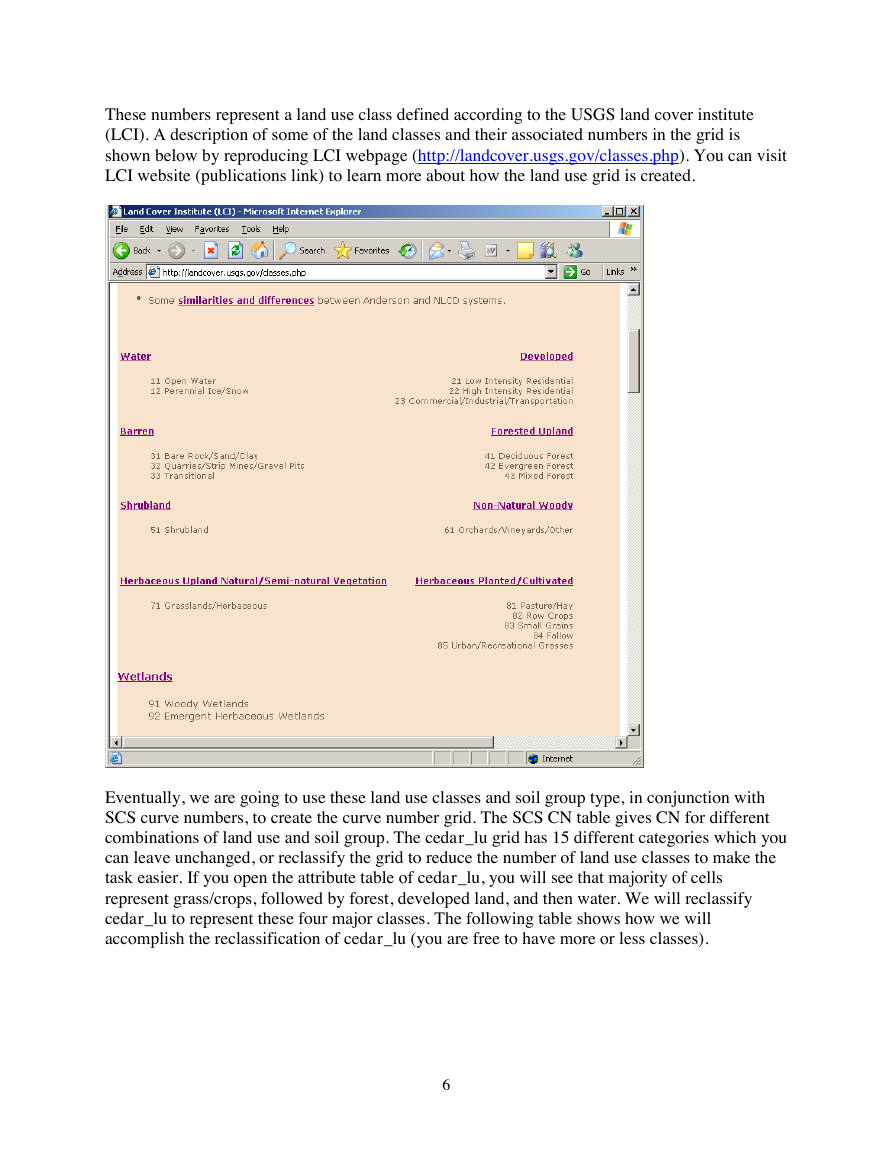
Add cedar_lu grid to the map document. You will see the grid is added with a unique symbology
assigned to cells having identical numbers as shown below:
5
�
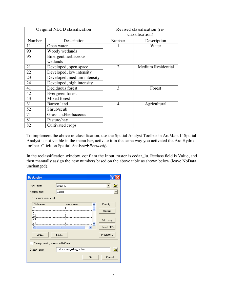
These numbers represent a land use class defined according to the USGS land cover institute
(LCI). A description of some of the land classes and their associated numbers in the grid is
shown below by reproducing LCI webpage (http://landcover.usgs.gov/classes.php). You can visit
LCI website (publications link) to learn more about how the land use grid is created.
Eventually, we are going to use these land use classes and soil group type, in conjunction with
SCS curve numbers, to create the curve number grid. The SCS CN table gives CN for different
combinations of land use and soil group. The cedar_lu grid has 15 different categories which you
can leave unchanged, or reclassify the grid to reduce the number of land use classes to make the
task easier. If you open the attribute table of cedar_lu, you will see that majority of cells
represent grass/crops, followed by forest, developed land, and then water. We will reclassify
cedar_lu to represent these four major classes. The following table shows how we will
accomplish the reclassification of cedar_lu (you are free to have more or less classes).
6
�
Original NLCD classification
Revised classification (re-
Description
classification)
Number
1
Description
Water
Number
11
90
95
2
3
Medium Residential
Open water
Woody wetlands
Emergent herbaceous
wetlands
Developed, open space
Developed, low intensity
Developed, medium intensity
Developed, high intensity
Deciduous forest
Evergreen forest
Mixed forest
Barren land
Shrub/scub
Grassland/herbaceous
Pasture/hay
Cultivated crops
21
22
23
24
41
42
43
31
52
71
81
82
To implement the above re-classification, use the Spatial Analyst Toolbar in ArcMap. If Spatial
Analyst is not visible in the menu bar, activate it in the same way you activated the Arc Hydro
toolbar. Click on Spatial AnalystReclassify….
In the reclassification window, confirm the Input raster is cedar_lu, Reclass field is Value, and
then manually assign the new numbers based on the above table as shown below (leave NoData
unchanged).
Agricultural
4
Forest
7
�
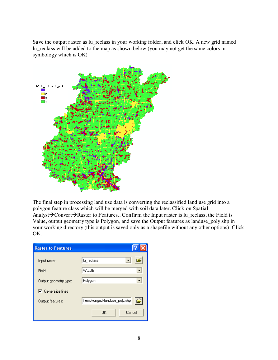
Save the output raster as lu_reclass in your working folder, and click OK. A new grid named
lu_reclass will be added to the map as shown below (you may not get the same colors in
symbology which is OK)
The final step in processing land use data is converting the reclassified land use grid into a
polygon feature class which will be merged with soil data later. Click on Spatial
AnalystConvertRaster to Features.. Confirm the Input raster is lu_reclass, the Field is
Value, output geometry type is Polygon, and save the Output features as landuse_poly.shp in
your working directory (this output is saved only as a shapefile without any other options). Click
OK.
8
�





 2023年江西萍乡中考道德与法治真题及答案.doc
 2012年重庆南川中考生物真题及答案.doc
 2013年江西师范大学地理学综合及文艺理论基础考研真题.doc
 2020年四川甘孜小升初语文真题及答案I卷.doc
 2020年注册岩土工程师专业基础考试真题及答案.doc
 2023-2024学年福建省厦门市九年级上学期数学月考试题及答案.doc
 2021-2022学年辽宁省沈阳市大东区九年级上学期语文期末试题及答案.doc
 2022-2023学年北京东城区初三第一学期物理期末试卷及答案.doc
 2018上半年江西教师资格初中地理学科知识与教学能力真题及答案.doc
 2012年河北国家公务员申论考试真题及答案-省级.doc
 2020-2021学年江苏省扬州市江都区邵樊片九年级上学期数学第一次质量检测试题及答案.doc
 2022下半年黑龙江教师资格证中学综合素质真题及答案.doc