Matlab生成视差图.pdf-资料库

Open videostereo.m in the Editor Run in the Command Window Stereo Vision Stereo vision is the process of recovering depth from camera images by comparing two or more views of the same scene. Simple, binocular stereo uses only two images, typically taken with parallel cameras that were separated by a horizontal distance known as the "baseline." The output of the stereo computation is a disparity map (which is translatable to a range image) which tells how far each point in the physical scene was from the camera. In this demo, we use MATLAB® and the Video and Image Processing Blockset™ to compute the depth map between two rectified stereo images. See the Image Rectification Demo to learn about the details behind rectification. In this demo we use block matching, which is the standard algorithm for highspeed stereo vision in hardware systems [8]. We first explore basic block matching, and then apply dynamic programming to improve accuracy, and image pyramiding to improve speed. This demo is similar to the Simulink Estimation for Stereo Vision Demo. The main difference is that the Simulink demo does not assume it has been given rectified images, and so searches along general epipolar lines that are not necessarily parallel to the xaxis. Contents Step 1. Read stereo image pair Step 2. Basic block matching Step 3. Subpixel estimation Step 4. Dynamic programming Step 5. Image Pyramiding Step 6. Combined pyramiding and dynamic programming Step 7. Backprojection References Step 1. Read stereo image pair Here we read in the color stereo image pair and convert the images to grayscale for the matching process. Using color images may provide some improvement in accuracy, but it is more efficient to work with only onechannel images. For this we use the ImageDataTypeConverter and the ColorSpaceConverter System objects. Below we show the left camera image and a color composite of both images so that one can easily see the disparity between them. hIdtc = video.ImageDataTypeConverter; hCsc = video.ColorSpaceConverter('Conversion','RGB to intensity'); leftI3chan = step(hIdtc,imread('vipstereo_hallwayLeft.png')); leftI = step(hCsc,leftI3chan); rightI3chan = step(hIdtc,imread('vipstereo_hallwayRight.png')); rightI = step(hCsc,rightI3chan); figure(1), clf; imshow(rightI3chan), title('Right image'); figure(2), clf; imshow(cat(3,rightI,leftI,leftI)), axis image; title('Color composite (right=red, left=cyan)');

Step 2. Basic block matching Next we perform basic block matching. For every pixel in the right image, we extract the 7 by7pixel block around it and search along the same row in the left image for the block that best matches it. Here we search in a range of pixels around the pixel's location in the first image, and we use the sum of absolute differences (SAD) to compare the image regions. We need only search over columns and not over rows because the images are rectified. We use the TemplateMatcher System object to perform this block matching between each block and the region of interest.

Dbasic = zeros(size(leftI), 'single'); disparityRange = 15; % Selects (2*halfBlockSize+1)‐by‐(2*halfBlockSize+1) block. halfBlockSize = 3; blockSize = 2*halfBlockSize+1; % Allocate space for all template matchers. tmats = cell(blockSize); % Scan over all rows. for m=1:size(leftI,1) % Set min/max row bounds for image block. minr = max(1,m‐halfBlockSize); maxr = min(size(leftI,1),m+halfBlockSize); % Scan over all columns. for n=1:size(leftI,2) minc = max(1,n‐halfBlockSize); maxc = min(size(leftI,2),n+halfBlockSize); % Compute disparity bounds. mind = max( ‐disparityRange, 1‐minc ); maxd = min( disparityRange, size(leftI,2)‐maxc ); % Construct template and region of interest. template = rightI(minr:maxr,minc:maxc); templateCenter = floor((size(template)+1)/2); roi = [minr+templateCenter(1)‐2 ... minc+templateCenter(2)+mind‐2 ... 1 maxd‐mind+1]; % Lookup proper TemplateMatcher object; create if empty. if isempty(tmats{size(template,1),size(template,2)}) tmats{size(template,1),size(template,2)} = ... video.TemplateMatcher('ROIInputPort',true); end thisTemplateMatcher = tmats{size(template,1),size(template,2)}; % Run TemplateMatcher object. 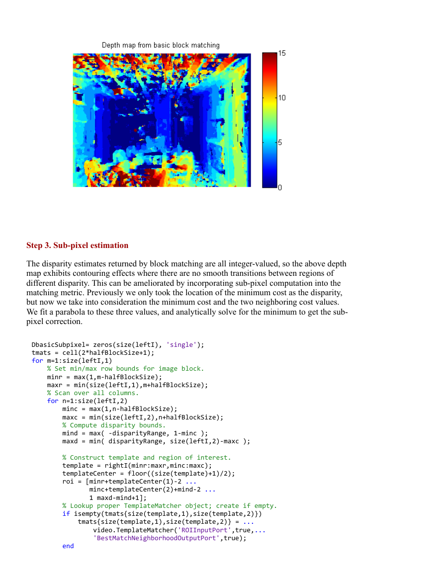loc = step(thisTemplateMatcher, leftI, template, roi); Dbasic(m,n) = loc(2) ‐ roi(2) + mind; end end In the results below, the basic block matching does well, as the correct shape of the stereo scene is recovered. However, there are noisy patches and bad depth estimates everywhere, especially on the ceiling. These are caused when no strong image features appear inside of the 7by7pixel windows being compared. Then the matching process is subject to noise since each pixel chooses its disparity independently of all the other pixels. For display purposes, we saturate the depth map to have only positive values. In general, slight angular misalignment of the stereo cameras used for image acquisition can allow both positive and negative disparities to appear validly in the depth map. In this case, however, the stereo cameras were near perfectly parallel, so the true disparities have only one sign. Thus this correction is valid. figure(3), clf; imshow(Dbasic,[]), axis image, colormap('jet'), colorbar; caxis([0 disparityRange]); title('Depth map from basic block matching');

Step 3. Subpixel estimation The disparity estimates returned by block matching are all integervalued, so the above depth map exhibits contouring effects where there are no smooth transitions between regions of different disparity. This can be ameliorated by incorporating subpixel computation into the matching metric. Previously we only took the location of the minimum cost as the disparity, but now we take into consideration the minimum cost and the two neighboring cost values. We fit a parabola to these three values, and analytically solve for the minimum to get the sub pixel correction. DbasicSubpixel= zeros(size(leftI), 'single'); tmats = cell(2*halfBlockSize+1); for m=1:size(leftI,1) % Set min/max row bounds for image block. minr = max(1,m‐halfBlockSize); maxr = min(size(leftI,1),m+halfBlockSize); % Scan over all columns. for n=1:size(leftI,2) minc = max(1,n‐halfBlockSize); maxc = min(size(leftI,2),n+halfBlockSize); % Compute disparity bounds. mind = max( ‐disparityRange, 1‐minc ); maxd = min( disparityRange, size(leftI,2)‐maxc ); % Construct template and region of interest. template = rightI(minr:maxr,minc:maxc); templateCenter = floor((size(template)+1)/2); roi = [minr+templateCenter(1)‐2 ... minc+templateCenter(2)+mind‐2 ... 1 maxd‐mind+1]; % Lookup proper TemplateMatcher object; create if empty. if isempty(tmats{size(template,1),size(template,2)}) tmats{size(template,1),size(template,2)} = ... video.TemplateMatcher('ROIInputPort',true,... 'BestMatchNeighborhoodOutputPort',true); end

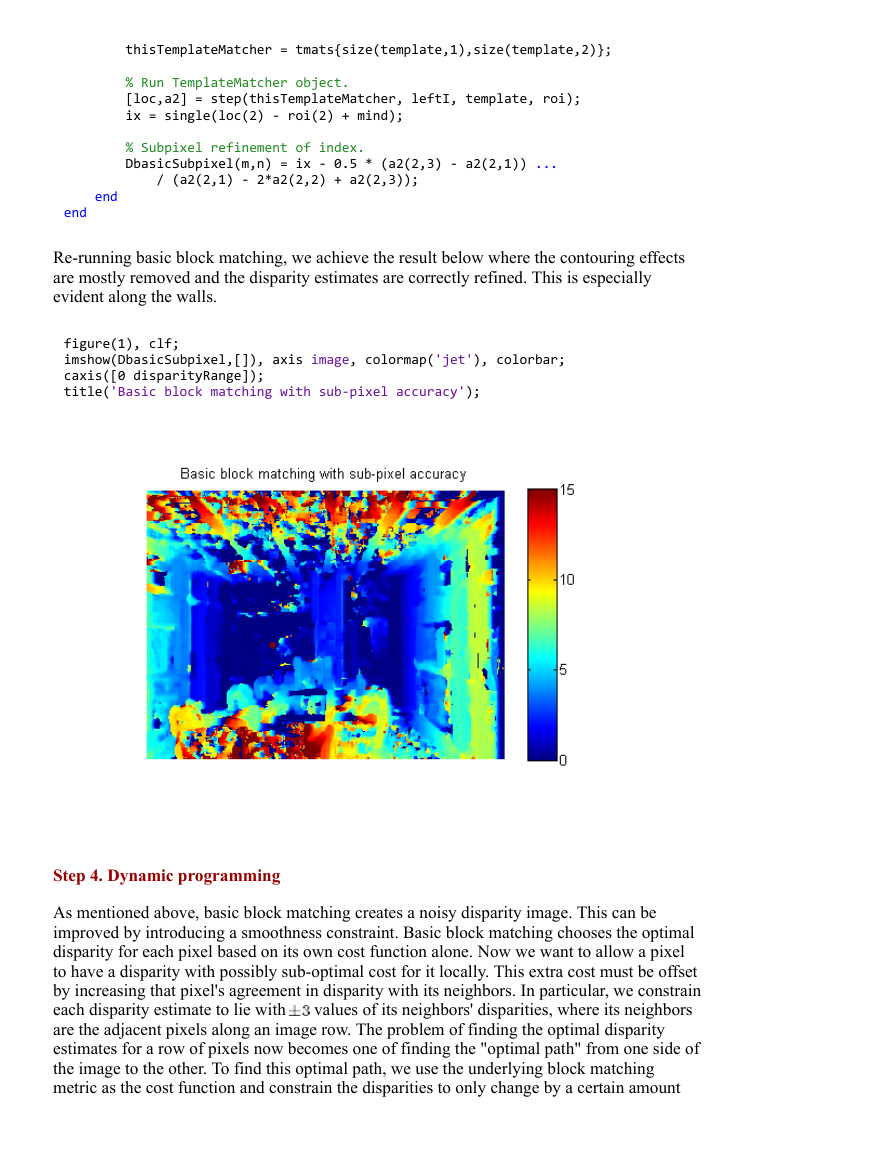
thisTemplateMatcher = tmats{size(template,1),size(template,2)}; % Run TemplateMatcher object. [loc,a2] = step(thisTemplateMatcher, leftI, template, roi); ix = single(loc(2) ‐ roi(2) + mind); % Subpixel refinement of index. DbasicSubpixel(m,n) = ix ‐ 0.5 * (a2(2,3) ‐ a2(2,1)) ... / (a2(2,1) ‐ 2*a2(2,2) + a2(2,3)); end end Rerunning basic block matching, we achieve the result below where the contouring effects are mostly removed and the disparity estimates are correctly refined. This is especially evident along the walls. figure(1), clf; imshow(DbasicSubpixel,[]), axis image, colormap('jet'), colorbar; caxis([0 disparityRange]); title('Basic block matching with sub‐pixel accuracy'); Step 4. Dynamic programming As mentioned above, basic block matching creates a noisy disparity image. This can be improved by introducing a smoothness constraint. Basic block matching chooses the optimal disparity for each pixel based on its own cost function alone. Now we want to allow a pixel to have a disparity with possibly suboptimal cost for it locally. This extra cost must be offset by increasing that pixel's agreement in disparity with its neighbors. In particular, we constrain each disparity estimate to lie with values of its neighbors' disparities, where its neighbors are the adjacent pixels along an image row. The problem of finding the optimal disparity estimates for a row of pixels now becomes one of finding the "optimal path" from one side of the image to the other. To find this optimal path, we use the underlying block matching metric as the cost function and constrain the disparities to only change by a certain amount

between adjacent pixels. This is a problem that can be solved efficiently using the technique of dynamic programming [3,4]. Ddynamic = zeros(size(leftI), 'single'); finf = 1e3; % False infinity disparityCost = finf*ones(size(leftI,2), 2*disparityRange + 1, 'single'); disparityPenalty = 0.5; % Penalty for disparity disagreement between pixels % Scan over all rows. for m=1:size(leftI,1) disparityCost(:) = finf; % Set min/max row bounds for image block. minr = max(1,m‐halfBlockSize); maxr = min(size(leftI,1),m+halfBlockSize); % Scan over all columns. for n=1:size(leftI,2) minc = max(1,n‐halfBlockSize); maxc = min(size(leftI,2),n+halfBlockSize); % Compute disparity bounds. mind = max( ‐disparityRange, 1‐minc ); maxd = min( disparityRange, size(leftI,2)‐maxc ); % Compute and save all matching costs. for d=mind:maxd disparityCost(n, d + disparityRange + 1) = ... sum(sum(abs(leftI(minr:maxr,(minc:maxc)+d) ... ‐ rightI(minr:maxr,minc:maxc)))); end end % Process scanline disparity costs with dynamic programming. optimalIndices = zeros(size(disparityCost), 'single'); cp = disparityCost(end,:); for j=size(disparityCost,1)‐1:‐1:1 % False infinity for this level cfinf = (size(disparityCost,1) ‐ j + 1)*finf; % Construct matrix for finding optimal move for each column % individually. [v,ix] = min([cfinf cfinf cp(1:end‐4)+3*disparityPenalty; cfinf cp(1:end‐3)+2*disparityPenalty; cp(1:end‐2)+disparityPenalty; cp(2:end‐1); cp(3:end)+disparityPenalty; cp(4:end)+2*disparityPenalty cfinf; cp(5:end)+3*disparityPenalty cfinf cfinf],[],1); cp = [cfinf disparityCost(j,2:end‐1)+v cfinf]; % Record optimal routes. optimalIndices(j,2:end‐1) = (2:size(disparityCost,2)‐1) + (ix ‐ 4); end % Recover optimal route. [~,ix] = min(cp); Ddynamic(m,1) = ix; for k=1:size(Ddynamic,2)‐1 Ddynamic(m,k+1) = optimalIndices(k, ... 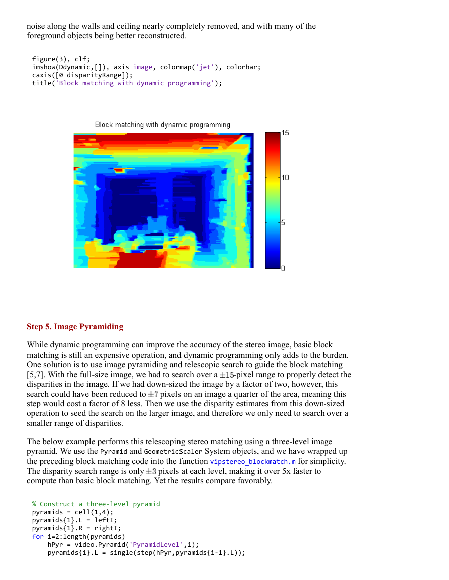max(1, min(size(optimalIndices,2), round(Ddynamic(m,k)) ) ) ); end end Ddynamic = Ddynamic ‐ disparityRange ‐ 1; The image below shows the stereo result refined by applying dynamic programming to each row individually. Dynamic programming does introduce errors of its own by blurring the edges around object boundaries due to the smoothness constraint. Also, it does nothing to smooth ''between'' rows, which is why a striation pattern now appears on the left side foreground chair. Despite these limitations, the result is significantly improved, with the

noise along the walls and ceiling nearly completely removed, and with many of the foreground objects being better reconstructed. figure(3), clf; imshow(Ddynamic,[]), axis image, colormap('jet'), colorbar; caxis([0 disparityRange]); title('Block matching with dynamic programming'); Step 5. Image Pyramiding While dynamic programming can improve the accuracy of the stereo image, basic block matching is still an expensive operation, and dynamic programming only adds to the burden. One solution is to use image pyramiding and telescopic search to guide the block matching [5,7]. With the fullsize image, we had to search over a disparities in the image. If we had downsized the image by a factor of two, however, this search could have been reduced to pixels on an image a quarter of the area, meaning this step would cost a factor of 8 less. Then we use the disparity estimates from this downsized operation to seed the search on the larger image, and therefore we only need to search over a smaller range of disparities. 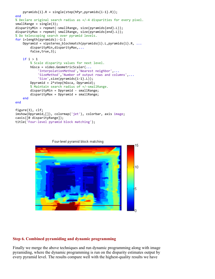pixel range to properly detect the The below example performs this telescoping stereo matching using a threelevel image pyramid. We use the Pyramid and GeometricScaler System objects, and we have wrapped up the preceding block matching code into the function vipstereo_blockmatch.m for simplicity. The disparity search range is only compute than basic block matching. Yet the results compare favorably. pixels at each level, making it over 5x faster to % Construct a three‐level pyramid pyramids = cell(1,4); pyramids{1}.L = leftI; pyramids{1}.R = rightI; for i=2:length(pyramids) hPyr = video.Pyramid('PyramidLevel',1); pyramids{i}.L = single(step(hPyr,pyramids{i‐1}.L));

pyramids{i}.R = single(step(hPyr,pyramids{i‐1}.R)); end % Declare original search radius as +/‐4 disparities for every pixel. smallRange = single(3); disparityMin = repmat(‐smallRange, size(pyramids{end}.L)); disparityMax = repmat( smallRange, size(pyramids{end}.L)); % Do telescoping search over pyramid levels. for i=length(pyramids):‐1:1 Dpyramid = vipstereo_blockmatch(pyramids{i}.L,pyramids{i}.R, ... disparityMin,disparityMax,... false,true,3); if i > 1 % Scale disparity values for next level. hGsca = video.GeometricScaler(... 'InterpolationMethod','Nearest neighbor',... 'SizeMethod','Number of output rows and columns',... 'Size',size(pyramids{i‐1}.L)); Dpyramid = 2*step(hGsca, Dpyramid); % Maintain search radius of +/‐smallRange. disparityMin = Dpyramid ‐ smallRange; disparityMax = Dpyramid + smallRange; end end figure(3), clf; imshow(Dpyramid,[]), colormap('jet'), colorbar, axis image; caxis([0 disparityRange]); title('Four‐level pyramid block matching'); Step 6. Combined pyramiding and dynamic programming Finally we merge the above techniques and run dynamic programming along with image pyramiding, where the dynamic programming is run on the disparity estimates output by every pyramid level. The results compare well with the highestquality results we have

资料库

Matlab生成视差图.pdf

相关推荐

人工智能

热门标签

最新资料