174
IEEE TRANSACTIONS ON SYSTEMS, MAN, AND CYBERNETICS—PART B: CYBERNETICS, VOL. 38, NO. 1, FEBRUARY 2008
Human Visual System-Based Image Enhancement
and Logarithmic Contrast Measure
Karen A. Panetta, Fellow, IEEE, Eric J. Wharton, Student Member, IEEE, and
Sos S. Agaian, Senior Member, IEEE
Abstract—Varying scene illumination poses many challenging
problems for machine vision systems. One such issue is develop-
ing global enhancement methods that work effectively across the
varying illumination. In this paper, we introduce two novel image
enhancement algorithms: edge-preserving contrast enhancement,
which is able to better preserve edge details while enhancing
contrast in images with varying illumination, and a novel multi-
histogram equalization method which utilizes the human visual
system (HVS) to segment the image, allowing a fast and ef-
ficient correction of nonuniform illumination. We then extend
this HVS-based multihistogram equalization approach to create a
general enhancement method that can utilize any combination of
enhancement algorithms for an improved performance. Addition-
ally, we propose new quantitative measures of image enhancement,
called the logarithmic Michelson contrast measure (AME) and the
logarithmic AME by entropy. Many image enhancement methods
require selection of operating parameters, which are typically
chosen using subjective methods, but these new measures allow
for automated selection. We present experimental results for these
methods and make a comparison against other leading algorithms.
Index Terms—Enhancement measure, human visual system
(HVS), image enhancement, logarithmic image processing.
I. INTRODUCTION
P ROVIDING digital images with good contrast and detail
is required for many important areas such as vision, re-
mote sensing, dynamic scene analysis, autonomous navigation,
and biomedical image analysis [3]. Producing visually nat-
ural images or modifying an image to better show the visual
information contained within the image is a requirement for
nearly all vision and image processing methods [9]. Methods
for obtaining such images from lower quality images are called
image enhancement techniques. Much effort has been spent in
extracting information from properly enhanced images [1], [2],
[4]–[8]. The enhancement task, however, is complicated by the
lack of any general unifying theory of image enhancement as
well as the lack of an effective quantitative standard of image
Manuscript received February 26, 2007; revised June 8, 2007. This work was
supported in part by the National Science Foundation under Award 0306464.
This paper was recommended by Associate Editor P. Bhattacharya.
K. A. Panetta and E. J. Wharton are with the Department of Electrical and
Computer Engineering, Tufts University, Medford, MA 02155 USA (e-mail:
karen@eecs.tufts.edu; ewhart02@eecs.tufts.edu).
S. S. Agaian is with the College of Engineering, University of Texas at
San Antonio, San Antonio, TX 78249 USA, and also with the Department of
Electrical and Computer Engineering, Tufts University, Medford, MA 02155
USA (e-mail: sos.agaian@utsa.edu).
Color versions of one or more of the figures in this paper are available online
at http://ieeexplore.ieee.org.
Digital Object Identifier 10.1109/TSMCB.2007.909440
quality to act as a design criterion for an image enhancement
system.
Furthermore, many enhancement algorithms have external
parameters which are sometimes difficult to fine-tune [11].
Most of these techniques are globally dependent on the type
of input and treat images instead of adapting to local features
within different regions [12]. A successful automatic image
enhancement requires an objective criterion for enhancement
and an external evaluation of quality [9].
Recently, several models of the human visual system (HVS)
have been used for image enhancement. One method is to
attempt to model the transfer functions of the parts of the HVS,
such as the optical nerve, cortex, and so forth. This method then
attempts to implement filters which recreate these processes to
model human vision [41], [42]. Another method uses a single
channel to model the entire system, processing the image with
a global algorithm [42].
HVS-based image enhancement aims to emulate the way in
which the HVS discriminates between useful and useless data
[34]. Weber’s Contrast Law quantifies the minimum change
required for the HVS to perceive contrast; however, this only
holds for a properly illuminated area. The minimum change
required is a function of background illumination and can
be closely approximated with three regions. The first is the
Devries–Rose region, which approximates this threshold for
under-illuminated areas. The second and most well known
region is the Weber region, which models this threshold for
properly illuminated areas. Finally, there is the saturation re-
gion, which approximates the threshold for over-illuminated
areas [33]. Each of these regions can be separately enhanced
and recombined to form a more visually pleasing output image.
In this paper, we propose a solution to these image enhance-
ment problems. The HVS system of image enhancement first
utilizes a method which segments the image into three regions
with similar qualities, allowing enhancement methods to be
adapted to the local features. This segmentation is based upon
models of the HVS.
The HVS system uses an objective evaluation measure for
selection of parameters. This allows for more consistent re-
sults while reducing the time required for the enhancement
process. The performance measure utilizes established methods
of measuring contrast and processes these values to assess the
useful information contained in the image. Operating para-
meters are selected by performing the enhancement with all
practical values of the parameters, by assessing each output
image using the measure, and by organizing these results into
a graph of performance measure versus parameters, where the
best parameters are located at local extrema.
1083-4419/$25.00 © 2007 IEEE
�
PANETTA et al.: HUMAN VISUAL SYSTEM-BASED IMAGE ENHANCEMENT
175
This paper is organized as follows. Section II presents
the necessary background information, including the parame-
terized logarithmic image processing (PLIP) model operator
primitives, used to achieve a better image enhancement, several
enhancement algorithms, including modified alpha rooting and
logarithmic enhancement, and the multiscale center-surround
Retinex algorithm, which we use for comparison purposes.
Section III presents new contrast measures, such as the logarith-
mic Michelson contrast measure (AME) and logarithmic AME
by entropy (AMEE), and a comparison with other measures
used in practice, such as the measure of image enhancement
(EME) and AME. Section IV introduces the new HVS-based
segmentation algorithms, including HVS-based multihistogram
equalization and HVS-based image enhancement. Section V
discusses in detail several new enhancement algorithms, includ-
ing edge-preserving contrast enhancement (EPCE) and the log-
arithm and AME-based weighted passband (LAW) algorithm.
Section VI presents a computational analysis comparing the
HVS algorithm to several state-of-the-art image enhancement
algorithms, such as low curvature image simplifier (LCIS).
Section VII presents the results of computer simulations and
analysis, comparing the HVS algorithm to Retinex and other
algorithms, showing that the HVS algorithm outperforms the
other algorithms. Section VIII discusses results and provides
some concluding comments.
II. BACKGROUND
In this section, the PLIP model, as well as several traditional
algorithms which will be used with the HVS-based image en-
hancement model, is discussed. These algorithms include modi-
fied alpha rooting and logarithmic enhancement [32], [38], [39].
A. PLIP Model and Arithmetic
It has been shown that there are five fundamental require-
ments for an image processing framework. First, it must be
based on a physically and/or psychophysically relevant image-
formation model. Second, its mathematical structures and oper-
ations must be both powerful and consistent with the physical
nature of the images. Third, its operations must be computa-
tionally effective. Fourth, it must be practically fruitful. Finally,
it must not damage either signal [13], [43].
An image representation on a computer must follow some
model that is physically consistent with a real-world image,
whether it is a photo, object, or scene [14]. Furthermore, the
arithmetic must be consistent with some real-world phenom-
enon, and it has been shown and is also intuitive that the HVS
should be considered when developing this model [15]. It is
important to consider which operations are to be used and why,
and that these effectively model and are physically consistent
with a real-world model for image processing [44], [45]. It
must also be shown that not only the image processing model is
mathematically well defined but also it must serve some useful
purpose. Finally, when a visually “good” image is added to
another visually “good” image, the resulting image must also
be “good” [43].
The PLIP model was introduced by Panetta et al. [43] to
provide a nonlinear framework for image processing, which
addresses these five requirements. It is designed to both main-
tain the pixel values inside the range (0,M] and more accurately
process images from an HVS point of view. To accomplish this,
images are processed as absorption filters using the gray tone
function. This gray tone function is as follows:
g(i, j) = M − f(i, j)
(1)
where f(i, j) is the original image function, g(i, j) is the output
gray tone function, and M is the maximum value of the range.
It can be seen that this gray tone function is much like a photo
negative.
The PLIP model operator primitives can be summarized as
follows:
c
1 − a
γ(M)
aΘb = k(M)
a ⊕ b = a + b − ab
γ(M)
a − b
k(M) − b
c ⊗ a = γ(M) − γ(M)
a ∗ b = ϕ
−1 (ϕ(a) · ϕ(b))
ϕ(a) = − λ(M) · lnβ
−1(a) = − λ(M) ·
ϕ
1 − exp
1/β
1 − f
λ(M)
−f
λ(M)
(2)
(3)
(4)
(5)
(6)
(7)
∗
where we use ⊕ as PLIP addition, Θ as PLIP subtraction, ⊗ as
as PLIP multiplication of
PLIP multiplication by a scalar, and
two images. Also, a and b are any gray tone pixel values, c is
a constant, M is the maximum value of the range, and β is a
constant. γ(M), k(M), and λ(M) are all arbitrary functions.
We use the linear case, such that they are functions of the type
γ(M) = AM + B, where A and B are integers; however, any
arbitrary function will work. In general, a and b correspond to
the same pixel in two different images that are being added,
subtracted, or multiplied. In [43], the best values of A and B
were experimentally determined to be any combination such
that γ(M), k(M), and λ(M) = 1026, and the best value of β
was determined to be β = 2.
B. Alpha Rooting and Logarithmic Enhancement
Alpha rooting is a straightforward method originally pro-
posed by Jain [54]. This enhancement algorithm was later
modified by Aghagolzadeh and Ersoy [40], as well as by Agaian
et al. [38], [39]. Alpha rooting is an algorithm that can be used
in combination with many different orthogonal transforms such
as the Fourier, Hartley, Haar wavelet, and cosine transforms.
The resulting output shows an emphasis on the high-frequency
content of the image without changing the phase of the trans-
form coefficients, resulting in an overall contrast enhancement.
This enhancement, however, can sometimes result in ugly arti-
facts [37].
Alpha rooting and logarithmic enhancement are transform-
based enhancement methods [32]. This means that they first
�
176
IEEE TRANSACTIONS ON SYSTEMS, MAN, AND CYBERNETICS—PART B: CYBERNETICS, VOL. 38, NO. 1, FEBRUARY 2008
perform some 2-D orthogonal transform on the input im-
age and then modify these transform coefficients. Alpha
rooting modifies the coefficients according to the following
formula:
O(p, s) = X(p, s) × |X(p, s)|α−1
(8)
where X(p, s) is the 2-D Fourier transform of the input image,
O(p, s) is the 2-D Fourier transform of the output image, and α
is a user-defined operating parameter with range 0 < α < 1.
Logarithmic enhancement was introduced by Agaian in [32],
[38], and [39]. This method also reduces the transform coef-
ficient magnitudes while leaving the phase unchanged, using
a logarithmic rule. Logarithmic enhancement uses two para-
meters, namely, β and λ. It works according to the following
transfer function:
|X(p, s)|λ + 1
O(p, s) = logβ
as a preprocessing step for other image processing purposes
such as object detection, classification, and recognition.
There is no universal measure which can specify both the
objective and subjective validity of the enhancement method
[22]. However, in [16], the three necessary characteristics of
a performance measure are given. First, it must measure the
desired characteristic in some holistic way. In our case, this
is contrast. Second, it must show a proportional relationship
between increase and decrease of this characteristic. Finally, it
must have some resulting characteristic to find optimal points.
One example of this is using local extrema. In this section,
we analyze the commonly used performance measures and
present two new quantitative contrast measures, called the
logarithmic AME and logarithmic AMEE, to address these
three characteristics. Since we are measuring improvement in
enhancement based on contrast, we will use enhancement and
contrast measures interchangeably.
.
(9)
A. New Contrast Measure
N
C. Multiscale Center-Surround Retinex
The multiscale center-surround Retinex algorithm was de-
veloped by Jobson et al. [36]. This algorithm was developed
to attain lightness and color constancy for machine vision
applications. While there is no single complete definition for
the Retinex model, lightness and color constancy refer to the re-
silience of perceived color and lightness to spatial and spectral
illumination variations. Benefits of the Retinex algorithm in-
clude dynamic range compression and color independence from
the special distribution of the scene illumination. However, this
algorithm can result in “halo” artifacts, especially in boundaries
between large uniform regions. Also, a “graying out” can occur,
in which the scene tends to change to middle gray.
The Retinex algorithm works by processing the image with
a high-pass filter, using several different widths and averaging
the results together. The algorithm is executed as follows:
R(i, j) =
wn log (I(i, j)) − log (F (i, j) ∗ I(i, j))
(10)
n=1
where I(i, j) is the input image, R(i, j) is the output image,
F (i, j) is a Gaussian kernel normalized to sum to one, wn is a
for this algorithm is the convolution
collection of weights, and
operator. In general, the weights wn are chosen to be equal. This
is a particular case of the Retinex algorithm.
∗
III. CONTRAST MEASURE AND PROPERTIES
An important step in a direct image enhancement approach
is to create a suitable performance measure. The improvement
found in the resulting images after enhancement is often very
difficult to measure. This problem becomes more apparent
when the enhancement algorithms are parametric, and one
needs to choose the best parameters, to choose the best trans-
form among a class of unitary transforms, or to automate the
image enhancement procedures. The problem becomes espe-
cially difficult when an image enhancement procedure is used
Many enhancement techniques are based on enhancing the
contrast of an image [17]–[20]. There have been many differing
definitions of an adequate measure of performance based on
contrast [21]–[23]. Gordon and Rangayan used local contrast
defined by the mean gray values in two rectangular win-
dows centered on a current pixel. Beghdadi and Negrate [21]
defined an improved version of the aforementioned measure
by basing their method on a local edge information of the
image. In the past, attempts at statistical measures of gray
level distribution of local contrast enhancement such as those
based on mean, variance, or entropy have not been particu-
larly useful or meaningful. A number of images, which show
an obvious contrast improvement, showed no consistency, as
a class, when using these statistical measurements. Morrow
et al. [23] introduced a measure based on the contrast his-
togram, which has a much greater consistency than statistical
measures.
Measures of enhancement based on the HVS have been
previously proposed [24]. Algorithms based on the HVS are
fundamental in computer vision [25]. Two definitions of con-
trast measure have traditionally been used for simple patterns
[26]: Michelson [27], [28], which is used for periodic patterns
like sinusoidal gratings, and Weber, which is used for large
uniform luminance backgrounds with small test targets [26].
However, these measures are not effective when applied to more
difficult scenarios such as images with nonuniform lighting or
shadows [26], [35]. The first practical use of a Weber’s-law-
based contrast measure, the image enhancement measure or
contrast measure, was developed by Agaian [30].
This contrast measure was later developed into the EME,
or measure of enhancement, and the EMEE, or measure of
enhancement by entropy [29], [31]. Finally, the Michelson Con-
trast Law was included to further improve the measures. These
were called the AME and AMEE [16]. These are summarized
in [16] and are calculated by dividing an image into k1 × k2
blocks, by calculating the measure for each block, and by
averaging the results as shown in the formula definitions.
In this paper, we capitalize on the strengths of these mea-
sures and improve upon them by including the PLIP operator
�
PANETTA et al.: HUMAN VISUAL SYSTEM-BASED IMAGE ENHANCEMENT
177
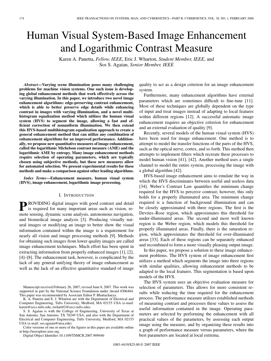
Fig. 1. Optimizing the logarithmic AMEE measure as given in (12) by choosing the best value for M. (a)–(c) Logarithmic AMEE graphs using M = 256,
M = 1026, and M = 4104, respectively. (d)–(f) Resulting images for alpha rooting using parameters from these graphs.
primitives. This allows for a more accurate processing of the
contrast information, as PLIP subtraction has been shown to
be consistent with Weber’s Contrast Law [13]. With these
modifications, we introduce the new logarithmic AME and
logarithmic AMEE measures, which are better able to assess
images and thus more accurately select parameters. These new
measures are presented in the following:
k2
j=1
1
20
i=1
⊗ k1
⊗ k1
1
k1k2
⊗ ln
1
k1k2
∗ ln
max:k,lΘI w
I w
⊕ I w
I w
k2
max:k,l
min:k,l
min:k,l
i=1
j=1
max:k,lΘI w
I w
⊕ I w
I w
max:k,l
min:k,l
min:k,l
log AMEk1k2(Φ) =
log AMEEk1k2(Φ) =
(11)
max:k,lΘI w
I w
⊕ I w
I w
max:k,l
min:k,l
min:k,l
.
(12)
To use the measures for selection of parameters, the algo-
rithm is first run for all practical values of the parameters. The
measure is calculated for each output image, and these data are
organized into a graph as measure versus parameters. Finally,
the best parameters are located at the local extrema.
B. Optimizing the PLIP for Contrast Measures
In [43], the PLIP model was optimized for image enhance-
ment procedures. However, for purposes of image enhancement
measures, these optimal values may be different. To address
this, an experiment was performed using a number of different
values for γ(M), k(M), and λ(M), as given in (2)–(7), using
the measures to select parameters for enhancement algorithms.
In this section, we present representative results of this exper-
iment to determine the optimal values of γ(M), k(M), and
λ(M).
Fig. 1 shows the results for the clock image using alpha
rooting. Fig. 1(a) shows the logarithmic AMEE graph using
M = 256, Fig. 1(b) shows the graph using M = 1026, and
Fig. 1(c) shows the graph for M = 4104, which is another
consistent value found in [43]. All of these graphs clearly
satisfy the three requirements stated earlier and are easy to read.
For all three graphs, the best value is located at a small peak
near the absolute minimum. This peak is most obvious in the
graph with M = 1026, occurring at α = 0.82. For the graph
with M = 256, this peak is located at α = 0.90, and for the
graph with M = 4104, this peak is located at α = 0.82. The
images with α = 0.82 are more visually pleasing, with better
contrast and definition. However, as M increases beyond 1026,
the curve smooths out, which can be seen in the graph with
M = 4104, until the peak is lost as M becomes sufficiently
large. This demonstrates that M = 1026 is the best value for
the contrast measures.
�
178
IEEE TRANSACTIONS ON SYSTEMS, MAN, AND CYBERNETICS—PART B: CYBERNETICS, VOL. 38, NO. 1, FEBRUARY 2008
Fig. 2. Choosing the best measure for the clock image. (a) EME, (b) EMEE, (c) AME, (d) AMEE, (e) logAME, and (f) logAMEE versus alpha graphs for the
clock using alpha rooting. (a), (c), (e), and (f) are the easiest to read, having only a few well-defined extrema to investigate for optimal enhancement parameter
alpha.
C. Selecting the Best Measure
In this section, we use the aforementioned enhancement
algorithms to select the best measure, which results in the most
visually pleasing image enhancement. While it is emphasized
in [16] that performance of a measure is algorithm dependent
and different measures will work best with different enhance-
ment algorithms, it is still possible to select which is best
for the general case. The algorithms have been performed for
numerous images using the measures presented in Section III to
select parameters. We visually compared the output images to
determine which measure is able to select the best parameters.
For this section, we show the results of alpha rooting and
logarithmic enhancement. We then present a summary for a
number of algorithms.
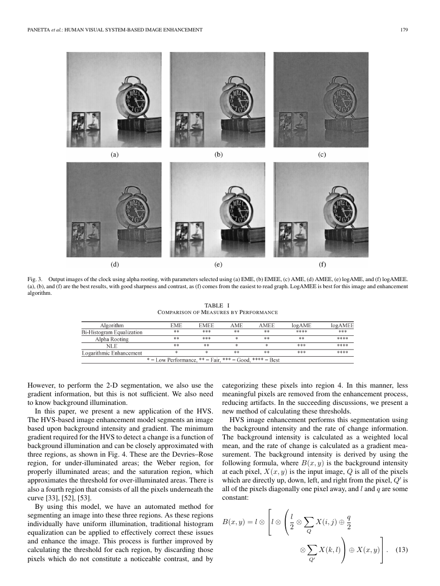
Figs. 2 and 3 show the process of selecting parameters using
the measures. Fig. 2 shows the resulting graphs generated by
processing the clock image with alpha rooting, plotting the
results of the measure against the values of α. Values are
selected as shown, which correspond to the local extrema in the
graphs. Fig. 3 shows the output images using the parameters
selected from these graphs.
As the graphs in Fig. 2 show, the output form of the PLIP-
based measures is smoother than the results of the measures
which utilize classical arithmetic. The logarithmic AMEE,
shown in Fig. 2(f), has only three local extrema. The EMEE and
AMEE graphs, shown in Fig. 2(b) and (d), have many peaks.
This makes the LogAMEE graph faster and easier to interpret,
as there are only three values to investigate. Also, as shown in
Fig. 3, the enhanced image using this value is visually more
pleasing than the others. It has the best balance of sharpness
and contrast, and there are no artifacts introduced.
Table I summarizes the results of this paper for all algorithms
used. It shows the averaged subjective evaluations of a number
of human interpreters. The algorithms were performed using
all six measures to select parameters, and the evaluators were
shown only the output images and were asked to rank them
between 1 and 1, with 4 being the best performance and 1 being
the lowest performance. The subjective evaluations show that
the new PLIP-based logarithmic AME and logarithmic AMEE
outperform the previously used measures.
IV. HVS-BASED SEGMENTATION
In this section, we propose a segmentation method based
upon the HVS. Several models of the HVS have been intro-
duced. One method attempts to model the transfer functions
of the parts of the HVS, such as the optical nerve, cortex,
and so forth. This method then attempts to implement filters
which recreate these processes to model human vision [41],
[42]. Another method uses a single channel to model the entire
system, processing the image with a global algorithm [42].
In [51], the authors use knowledge of the HVS to segment
an image into a number of subimages, each containing similar
1-D edge information. This is performed using a collection of
known 1-D curves. They show that, along with the gradient in-
formation along those curves, this is a complete representation
of the image. We expand upon this by segmenting an image into
a collection of 2-D images, all with similar internal properties.
�
PANETTA et al.: HUMAN VISUAL SYSTEM-BASED IMAGE ENHANCEMENT
179
Fig. 3. Output images of the clock using alpha rooting, with parameters selected using (a) EME, (b) EMEE, (c) AME, (d) AMEE, (e) logAME, and (f) logAMEE.
(a), (b), and (f) are the best results, with good sharpness and contrast, as (f) comes from the easiest to read graph. LogAMEE is best for this image and enhancement
algorithm.
COMPARISON OF MEASURES BY PERFORMANCE
TABLE I
However, to perform the 2-D segmentation, we also use the
gradient information, but this is not sufficient. We also need
to know background illumination.
In this paper, we present a new application of the HVS.
The HVS-based image enhancement model segments an image
based upon background intensity and gradient. The minimum
gradient required for the HVS to detect a change is a function of
background illumination and can be closely approximated with
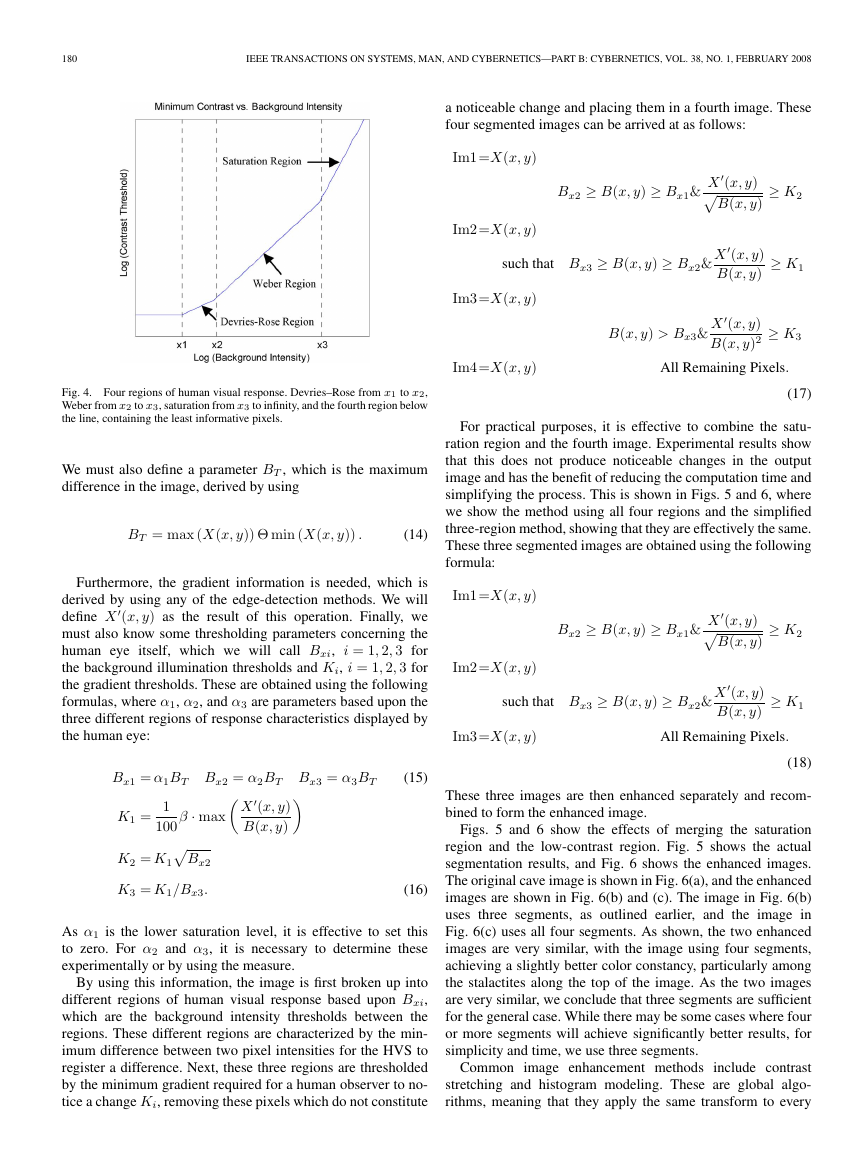
three regions, as shown in Fig. 4. These are the Devries–Rose
region, for under-illuminated areas;
the Weber region, for
properly illuminated areas; and the saturation region, which
approximates the threshold for over-illuminated areas. There is
also a fourth region that consists of all the pixels underneath the
curve [33], [52], [53].
By using this model, we have an automated method for
segmenting an image into these three regions. As these regions
individually have uniform illumination, traditional histogram
equalization can be applied to effectively correct these issues
and enhance the image. This process is further improved by
calculating the threshold for each region, by discarding those
pixels which do not constitute a noticeable contrast, and by
categorizing these pixels into region 4. In this manner, less
meaningful pixels are removed from the enhancement process,
reducing artifacts. In the succeeding discussions, we present a
new method of calculating these thresholds.
HVS image enhancement performs this segmentation using
the background intensity and the rate of change information.
The background intensity is calculated as a weighted local
mean, and the rate of change is calculated as a gradient mea-
surement. The background intensity is derived by using the
following formula, where B(x, y) is the background intensity
at each pixel, X(x, y) is the input image, Q is all of the pixels
is
which are directly up, down, left, and right from the pixel, Q
all of the pixels diagonally one pixel away, and l and q are some
constant:
l ⊗
l
2
B(x, y) = l ⊗
⊗
X(i, j) ⊕ q
2
⊕ X(x, y)
.
X(k, l)
Q
⊗
Q
(13)
�
180
IEEE TRANSACTIONS ON SYSTEMS, MAN, AND CYBERNETICS—PART B: CYBERNETICS, VOL. 38, NO. 1, FEBRUARY 2008
a noticeable change and placing them in a fourth image. These
four segmented images can be arrived at as follows:
≥ K2
≥ K1
≥ K3
Im1=X(x, y)
Im2=X(x, y)
Bx2 ≥ B(x, y) ≥ Bx1& X
(x, y)
B(x, y)
such that Bx3 ≥ B(x, y) ≥ Bx2& X
(x, y)
B(x, y)
Im3=X(x, y)
B(x, y) > Bx3& X
(x, y)
B(x, y)2
Im4=X(x, y)
All Remaining Pixels.
(17)
For practical purposes, it is effective to combine the satu-
ration region and the fourth image. Experimental results show
that this does not produce noticeable changes in the output
image and has the benefit of reducing the computation time and
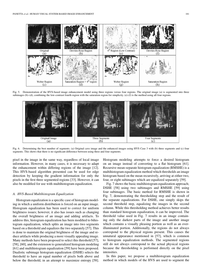
simplifying the process. This is shown in Figs. 5 and 6, where
we show the method using all four regions and the simplified
three-region method, showing that they are effectively the same.
These three segmented images are obtained using the following
formula:
≥ K2
≥ K1
Im1=X(x, y)
Im2=X(x, y)
Bx2 ≥ B(x, y) ≥ Bx1& X
(x, y)
B(x, y)
such that Bx3 ≥ B(x, y) ≥ Bx2& X
(x, y)
B(x, y)
Im3=X(x, y)
All Remaining Pixels.
(18)
These three images are then enhanced separately and recom-
bined to form the enhanced image.
Figs. 5 and 6 show the effects of merging the saturation
region and the low-contrast region. Fig. 5 shows the actual
segmentation results, and Fig. 6 shows the enhanced images.
The original cave image is shown in Fig. 6(a), and the enhanced
images are shown in Fig. 6(b) and (c). The image in Fig. 6(b)
uses three segments, as outlined earlier, and the image in
Fig. 6(c) uses all four segments. As shown, the two enhanced
images are very similar, with the image using four segments,
achieving a slightly better color constancy, particularly among
the stalactites along the top of the image. As the two images
are very similar, we conclude that three segments are sufficient
for the general case. While there may be some cases where four
or more segments will achieve significantly better results, for
simplicity and time, we use three segments.
Common image enhancement methods include contrast
stretching and histogram modeling. These are global algo-
rithms, meaning that they apply the same transform to every
Fig. 4. Four regions of human visual response. Devries–Rose from x1 to x2,
Weber from x2 to x3, saturation from x3 to infinity, and the fourth region below
the line, containing the least informative pixels.
We must also define a parameter BT , which is the maximum
difference in the image, derived by using
BT = max (X(x, y)) Θ min (X(x, y)) .
(14)
Furthermore, the gradient information is needed, which is
derived by using any of the edge-detection methods. We will
(x, y) as the result of this operation. Finally, we
define X
must also know some thresholding parameters concerning the
human eye itself, which we will call Bxi, i = 1, 2, 3 for
the background illumination thresholds and Ki, i = 1, 2, 3 for
the gradient thresholds. These are obtained using the following
formulas, where α1, α2, and α3 are parameters based upon the
three different regions of response characteristics displayed by
the human eye:
Bx1 = α1BT Bx2 = α2BT Bx3 = α3BT
(x, y)
X
B(x, y)
K1 =
1
100 β · max
K2 = K1
Bx2
K3 = K1/Bx3.
(15)
(16)
As α1 is the lower saturation level, it is effective to set this
to zero. For α2 and α3, it is necessary to determine these
experimentally or by using the measure.
By using this information, the image is first broken up into
different regions of human visual response based upon Bxi,
which are the background intensity thresholds between the
regions. These different regions are characterized by the min-
imum difference between two pixel intensities for the HVS to
register a difference. Next, these three regions are thresholded
by the minimum gradient required for a human observer to no-
tice a change Ki, removing these pixels which do not constitute
�
PANETTA et al.: HUMAN VISUAL SYSTEM-BASED IMAGE ENHANCEMENT
181
Fig. 5. Demonstration of the HVS-based image enhancement model using three regions versus four regions. The original image (a) is segmented into three
subimages (b)–(d), combining the low-contrast fourth region with the saturation region for simplicity. (e)-(f) is the method using all four regions.
Fig. 6. Determining the best number of segments. (a) Original cave image and the enhanced images using HVS Case 3 with (b) three segments and (c) four
segments. This shows that there is no significant difference between using three and four segments.
pixel in the image in the same way, regardless of local image
information. However, in many cases, it is necessary to adapt
the enhancement within differing regions of the image [12].
This HVS-based algorithm presented can be used for edge
detection by keeping the gradient information for only the
pixels in the first three segmented regions [33]. However, it can
also be modified for use with multihistogram equalization.
A. HVS-Based Multihistogram Equalization
Histogram equalization is a specific case of histogram model-
ing in which a uniform distribution is forced on an input image.
Histogram equalization has been used to correct for uniform
brightness issues; however, it also has issues such as changing
the overall brightness of an image and adding artifacts. To
address this, histogram equalization has been modified to bihis-
togram equalization, which splits an image into two segments
based on a threshold and equalizes the two separately [57]. This
is done to maintain the original brightness of the image and re-
duce artifacts while producing a more visually appealing image.
Many methods have been proposed to select this threshold [57],
[58], [60], and the extension to generalized histogram modeling
[61] and multihistogram equalization [59] have been proposed.
Dualistic subimage histogram equalization (DSHE) selects the
threshold to have an equal number of pixels both above and
below the threshold, in an attempt to maximize entropy [58].
Histogram modeling attempts to force a desired histogram
on an image instead of converting to a flat histogram [61].
Recursive mean-separate histogram equalization (RMSHE) is a
multihistogram equalization method which thresholds an image
histogram based on the mean recursively, arriving at either two,
four, or eight subimages which are equalized separately [59].
Fig. 7 shows the basic multihistogram equalization approach;
DSHE [58] using two subimages and RMSHE [59] using
four subimages. The basic method for RMSHE is shown in
Fig. 7, demonstrating the thresholding step and the result of
the separate equalizations. For DSHE, one simply skips the
second threshold step, equalizing the images in the second
column. While this thresholding method achieves better results
than standard histogram equalization, it can be improved. The
threshold value used in Fig. 7 results in an image contain-
ing only the darkest parts of the image and another image
which contains a visually pleasing portion as well as an over-
illuminated portion. Additionally, the regions do not always
correspond to the physical regions present. This causes the
unnatural appearance mentioned in [57], which is common
to histogram equalization methods. The segmented regions
still do not always correspond to the actual physical regions
because the thresholding is performed directly on the pixel
intensities.
In this paper, we propose a multihistogram equalization
method in which models of the HVS are used to segment the
�



 2023年江西萍乡中考道德与法治真题及答案.doc
 2012年重庆南川中考生物真题及答案.doc
 2013年江西师范大学地理学综合及文艺理论基础考研真题.doc
 2020年四川甘孜小升初语文真题及答案I卷.doc
 2020年注册岩土工程师专业基础考试真题及答案.doc
 2023-2024学年福建省厦门市九年级上学期数学月考试题及答案.doc
 2021-2022学年辽宁省沈阳市大东区九年级上学期语文期末试题及答案.doc
 2022-2023学年北京东城区初三第一学期物理期末试卷及答案.doc
 2018上半年江西教师资格初中地理学科知识与教学能力真题及答案.doc
 2012年河北国家公务员申论考试真题及答案-省级.doc
 2020-2021学年江苏省扬州市江都区邵樊片九年级上学期数学第一次质量检测试题及答案.doc
 2022下半年黑龙江教师资格证中学综合素质真题及答案.doc