The Relationship Between Precision-Recall and ROC Curves
Jesse Davis
Mark Goadrich
Department of Computer Sciences and Department of Biostatistics and Medical Informatics, University of
Wisconsin-Madison, 1210 West Dayton Street, Madison, WI, 53706 USA
jdavis@cs.wisc.edu
richm@cs.wisc.edu
Abstract
Receiver Operator Characteristic (ROC)
curves are commonly used to present re-
sults for binary decision problems in ma-
chine learning.
However, when dealing
with highly skewed datasets, Precision-Recall
(PR) curves give a more informative picture
of an algorithm’s performance. We show that
a deep connection exists between ROC space
and PR space, such that a curve dominates
in ROC space if and only if it dominates
in PR space. A corollary is the notion of
an achievable PR curve, which has proper-
ties much like the convex hull in ROC space;
we show an ecient algorithm for computing
this curve. Finally, we also note dierences
in the two types of curves are signicant for
algorithm design. For example, in PR space
it is incorrect to linearly interpolate between
points. Furthermore, algorithms that opti-
mize the area under the ROC curve are not
guaranteed to optimize the area under the
PR curve.
1. Introduction
In machine learning, current research has shifted away
from simply presenting accuracy results when perform-
ing an empirical validation of new algorithms. This is
especially true when evaluating algorithms that output
probabilities of class values. Provost et al. (1998) have
argued that simply using accuracy results can be mis-
leading. They recommended when evaluating binary
decision problems to use Receiver Operator Character-
istic (ROC) curves, which show how the number of cor-
rectly classied positive examples varies with the num-
ber of incorrectly classied negative examples. How-
ever, ROC curves can present an overly optimistic view
of an algorithm’s performance if there is a large skew
Appearing in Proceedings of the 23 rd International Con-
ference on Machine Learning, Pittsburgh, PA, 2006. Copy-
right 2006 by the author(s)/owner(s).
in the class distribution. Drummond and Holte (2000;
2004) have recommended using cost curves to address
this issue. Cost curves are an excellent alternative to
ROC curves, but discussing them is beyond the scope
of this paper.
Precision-Recall (PR) curves, often used in Informa-
tion Retrieval (Manning & Schutze, 1999; Raghavan
et al., 1989), have been cited as an alternative to ROC
curves for tasks with a large skew in the class dis-
tribution (Bockhorst & Craven, 2005; Bunescu et al.,
2004; Davis et al., 2005; Goadrich et al., 2004; Kok &
Domingos, 2005; Singla & Domingos, 2005). An im-
portant dierence between ROC space and PR space
is the visual representation of the curves. Looking
at PR curves can expose dierences between algo-
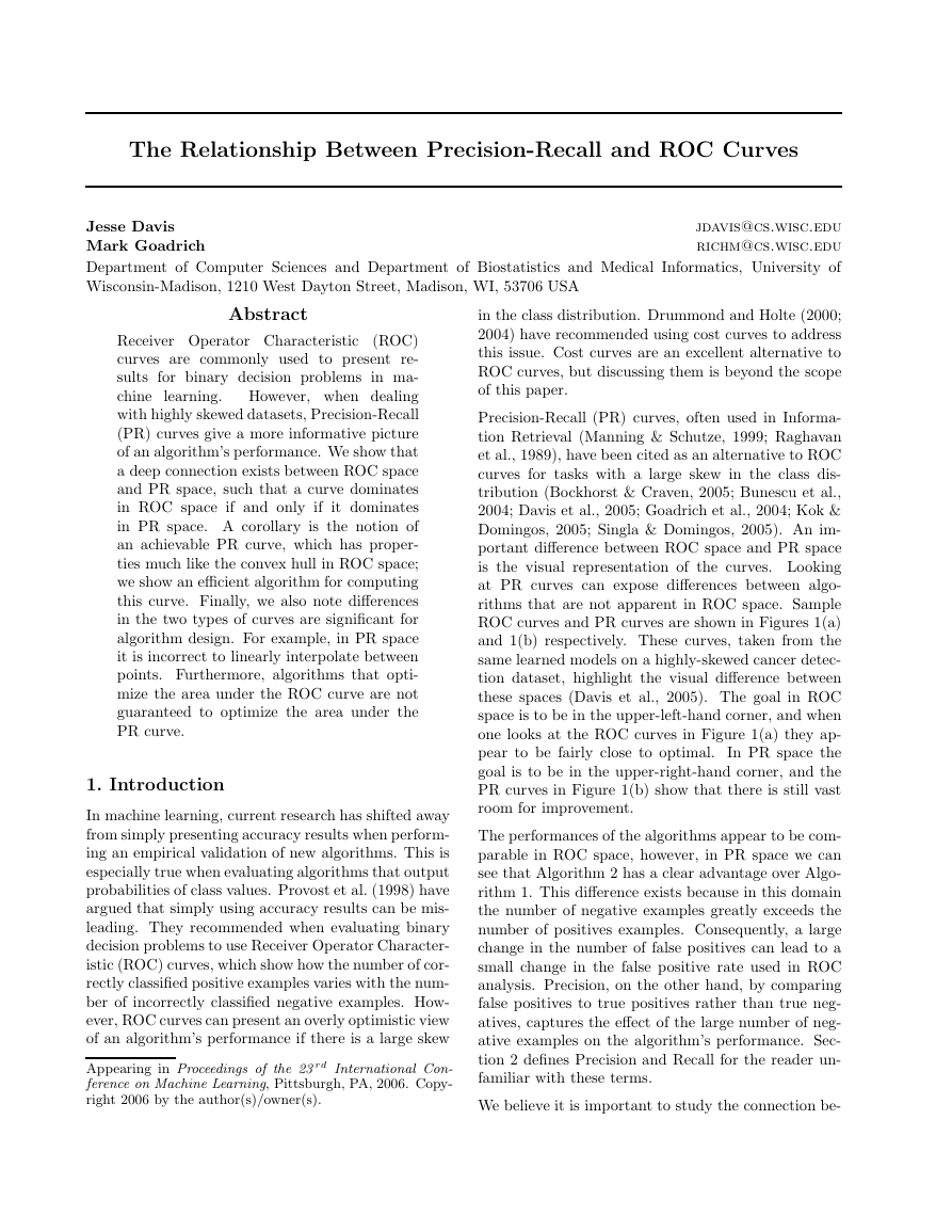
rithms that are not apparent in ROC space. Sample
ROC curves and PR curves are shown in Figures 1(a)
and 1(b) respectively. These curves, taken from the
same learned models on a highly-skewed cancer detec-
tion dataset, highlight the visual dierence between
these spaces (Davis et al., 2005). The goal in ROC
space is to be in the upper-left-hand corner, and when
one looks at the ROC curves in Figure 1(a) they ap-
pear to be fairly close to optimal.
In PR space the
goal is to be in the upper-right-hand corner, and the
PR curves in Figure 1(b) show that there is still vast
room for improvement.
The performances of the algorithms appear to be com-
parable in ROC space, however, in PR space we can
see that Algorithm 2 has a clear advantage over Algo-
rithm 1. This dierence exists because in this domain
the number of negative examples greatly exceeds the
number of positives examples. Consequently, a large
change in the number of false positives can lead to a
small change in the false positive rate used in ROC
analysis. Precision, on the other hand, by comparing
false positives to true positives rather than true neg-
atives, captures the eect of the large number of neg-
ative examples on the algorithm’s performance. Sec-
tion 2 denes Precision and Recall for the reader un-
familiar with these terms.
We believe it is important to study the connection be-
�
The Relationship Between Precision-Recall and ROC Curves
1
e
t
a
R
e
v
i
t
i
s
o
P
e
u
r
T
0.8
0.6
0.4
0.2
0
0
Algorithm 1
Algorithm 2
0.2 0.4 0.6 0.8
False Positive Rate
1
1
0.8
n
o
i
s
i
c
e
r
P
0.6
0.4
0.2
0
Algorithm 1
Algorithm 2
0
0.2 0.4 0.6 0.8
1
Recall
(a) Comparison in ROC space
(b) Comparison in PR space
Figure 1. The dierence between comparing algorithms in ROC vs PR space
tween these two spaces, and whether some of the in-
teresting properties of ROC space also hold for PR
space. We show that for any dataset, and hence a
xed number of positive and negative examples, the
ROC curve and PR curve for a given algorithm con-
tain the \same points." Therefore the PR curves for
Algorithm I and Algorithm II in Figure 1(b) are, in a
sense that we formally dene, equivalent to the ROC
curves for Algorithm I and Algorithm II, respectively
in Figure 1(a). Based on this equivalence for ROC and
PR curves, we show that a curve dominates in ROC
space if and only if it dominates in PR space. Sec-
ond, we introduce the PR space analog to the convex
hull in ROC space, which we call the achievable PR
curve. We show that due to the equivalence of these
two spaces we can eciently compute the achievable
PR curve. Third we demonstrate that in PR space
it is insucient to linearly interpolate between points.
Finally, we show that an algorithm that optimizes the
area under the ROC curve is not guaranteed to opti-
mize the area under the PR curve.
2. Review of ROC and Precision-Recall
In a binary decision problem, a classier labels ex-
amples as either positive or negative. The decision
made by the classier can be represented in a struc-
ture known as a confusion matrix or contingency ta-
ble. The confusion matrix has four categories: True
positives (TP) are examples correctly labeled as posi-
tives. False positives (FP) refer to negative examples
incorrectly labeled as positive. True negatives (TN)
correspond to negatives correctly labeled as negative.
Finally, false negatives (FN) refer to positive examples
incorrectly labeled as negative.
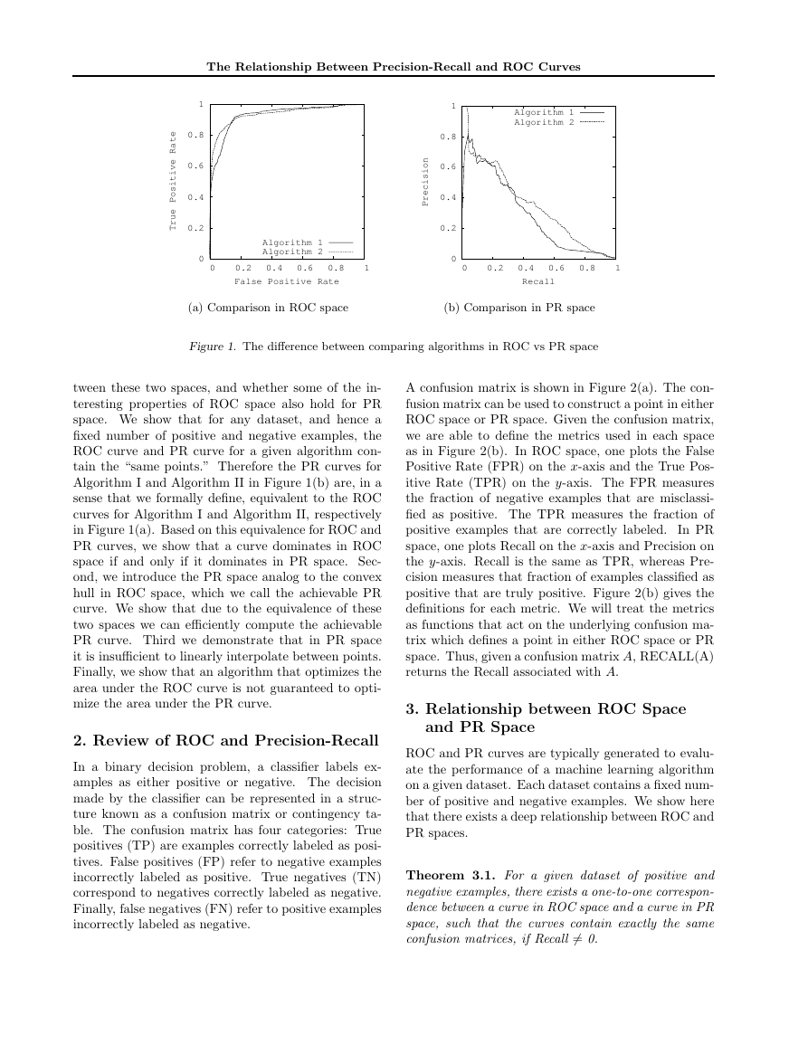
A confusion matrix is shown in Figure 2(a). The con-
fusion matrix can be used to construct a point in either
ROC space or PR space. Given the confusion matrix,
we are able to dene the metrics used in each space
as in Figure 2(b). In ROC space, one plots the False
Positive Rate (FPR) on the x-axis and the True Pos-
itive Rate (TPR) on the y-axis. The FPR measures
the fraction of negative examples that are misclassi-
ed as positive. The TPR measures the fraction of
positive examples that are correctly labeled.
In PR
space, one plots Recall on the x-axis and Precision on
the y-axis. Recall is the same as TPR, whereas Pre-
cision measures that fraction of examples classied as
positive that are truly positive. Figure 2(b) gives the
denitions for each metric. We will treat the metrics
as functions that act on the underlying confusion ma-
trix which denes a point in either ROC space or PR
space. Thus, given a confusion matrix A, RECALL(A)
returns the Recall associated with A.
3. Relationship between ROC Space
and PR Space
ROC and PR curves are typically generated to evalu-
ate the performance of a machine learning algorithm
on a given dataset. Each dataset contains a xed num-
ber of positive and negative examples. We show here
that there exists a deep relationship between ROC and
PR spaces.
Theorem 3.1. For a given dataset of positive and
negative examples, there exists a one-to-one correspon-
dence between a curve in ROC space and a curve in PR
space, such that the curves contain exactly the same
confusion matrices, if Recall 6= 0.
�
The Relationship Between Precision-Recall and ROC Curves
actual
positive
actual
negative
predicted positive
predicted negative
T P
F N
F P
T N
(a) Confusion Matrix
Recall
Precision
=
=
True Positive Rate =
False Positive Rate =
T P
T P +F N
T P
T P +F P
T P
T P +F N
F P
F P +T N
(b) Denitions of metrics
Figure 2. Common machine learning evaluation metrics
Proof. Note that a point in ROC space denes a
unique confusion matrix when the dataset is xed.
Since in PR space we ignore F N , one might worry
that each point may correspond to multiple confusion
matrices. However, with a xed number of positive
and negative examples, given the other three entries
in a matrix, F N is uniquely determined. If Recall =
0, we are unable to recover F P , and thus cannot nd
a unique confusion matrix.
Consequently, we have a one-to-one mapping between
confusion matrices and points in PR space. This im-
plies that we also have a one-to-one mapping between
points (each dened by a confusion matrix) in ROC
space and PR space; hence, we can translate a curve
in ROC space to PR space and vice-versa.
One important denition we need for our next theorem
is the notion that one curve dominates another curve,
\meaning that all other...curves are beneath it or equal
to it (Provost et al., 1998)."
Theorem 3.2. For a xed number of positive and neg-
ative examples, one curve dominates a second curve in
ROC space if and only if the rst dominates the second
in Precision-Recall space.
Proof.
Claim 1 ()):
If a curve dominates in ROC
space then it dominates in PR space. Proof by
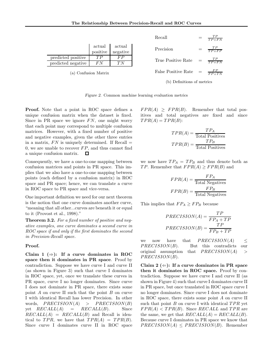
contradiction. Suppose we have curve I and curve II
(as shown in Figure 3) such that curve I dominates
in ROC space, yet, once we translate these curves in
PR space, curve I no longer dominates. Since curve
I does not dominate in PR space, there exists some
point A on curve II such that the point B on curve
I with identical Recall has lower Precision. In other
words, P RECISION (A) > P RECISION (B)
yet RECALL(A) = RECALL(B).
Since
RECALL(A) = RECALL(B) and Recall
is iden-
tical to T P R, we have that T P R(A) = T P R(B).
Since curve I dominates curve II in ROC space
F P R(A) F P R(B). Remember that total pos-
itives and total negatives are xed and since
T P R(A) = T P R(B):
T P R(A) =
T P R(B) =
T PA
Total Positives
T PB
Total Positives
we now have T PA = T PB and thus denote both as
T P . Remember that F P R(A) F P R(B) and
F P R(A) =
F P R(B) =
F PA
Total Negatives
F PB
Total Negatives
This implies that F PA F PB because
P RECISION (A) =
P RECISION (B) =
T P
F PA + T P
T P
F PB + T P
now
have
we
P RECISION (B).
original
P RECISION (B).
this
that
contradicts our
assumption that P RECISION (A) >
P RECISION (A)
But
Claim 2 ((): If a curve dominates in PR space
then it dominates in ROC space. Proof by con-
tradiction. Suppose we have curve I and curve II (as
shown in Figure 4) such that curve I dominates curve II
in PR space, but once translated in ROC space curve I
no longer dominates. Since curve I does not dominate
in ROC space, there exists some point A on curve II
such that point B on curve I with identical T P R yet
F P R(A) < T P R(B). Since RECALL and T P R are
the same, we get that RECALL(A) = RECALL(B).
Because curve I dominates in PR space we know that
P RECISION (A) P RECISION (B). Remember
�
The Relationship Between Precision-Recall and ROC Curves
e
t
a
R
e
v
i
t
i
s
o
P
e
u
r
T
1
0.8
0.6
B
A
0.4
0.2
0
0
Curve I
Curve II
0.2 0.4 0.6 0.8
False Positive Rate
1
e
t
a
R
e
v
i
t
i
s
o
P
e
u
r
T
1
0.8
0.6
0.4
B = A
0.2
0
0
Curve I
Curve II
0.2 0.4 0.6 0.8
False Positive Rate
1
(a) Case 1: F P R(A) > F P R(B)
(b) Case 2: F P R(A) = F P R(B)
Figure 3. Two cases for Claim 1 of Theorem 3.2
1
0.8
n
o
i
s
i
c
e
r
P
0.6
0.4
0.2
Curve I
Curve II
B
A
0
0
0.2 0.4 0.6 0.8
1
Recall
1
0.8
n
o
i
s
i
c
e
r
P
0.6
0.4
0.2
0
Curve I
Curve II
B = A
0
0.2 0.4 0.6 0.8
1
Recall
(a) Case 1: P RECI SI ON (A) <
P RECI SI ON (B)
(b) Case 2: P RECI SI ON (A) =
P RECI SI ON (B)
Figure 4. Two cases of Claim 2 of Theorem 3.2
that RECALL(A) = RECALL(B) and
we nd that F PA F PB. Now we have
RECALL(A) =
RECALL(B) =
T PA
Total Positives
T PB
Total Positives
We know that T PA = T PB, so we will now denote
them simply as T P . Because P RECISION (A)
P RECISION (B) and
P RECISION (A) =
P RECISION (B) =
T P
T P + F PA
T P
T P + F PB
F P R(A) =
F P R(B) =
F PA
Total Negatives
F PB
Total Negatives
This implies that F P R(A) F P R(B) and this con-
tradicts our original assumption that F P R(A) <
F P R(B):
In ROC space the convex hull is a crucial idea. Given
a set of points in ROC space, the convex hull must
meet the following three criteria:
1. Linear interpolation is used between adjacent
points.
2. No point lies above the nal curve.
�
The Relationship Between Precision-Recall and ROC Curves
1
e
t
a
R
e
v
i
t
i
s
o
P
e
u
r
T
0.8
0.6
0.4
0.2
1
e
t
a
R
e
v
i
t
i
s
o
P
e
u
r
T
0.8
0.6
0.4
0.2
0
0
0.2 0.4 0.6 0.8
False Positive Rate
1
0
0
0.2 0.4 0.6 0.8
False Positive Rate
1
1
0.8
n
o
i
s
i
c
e
r
P
0.6
0.4
0.2
0
0
0.2 0.4 0.6 0.8
1
Recall
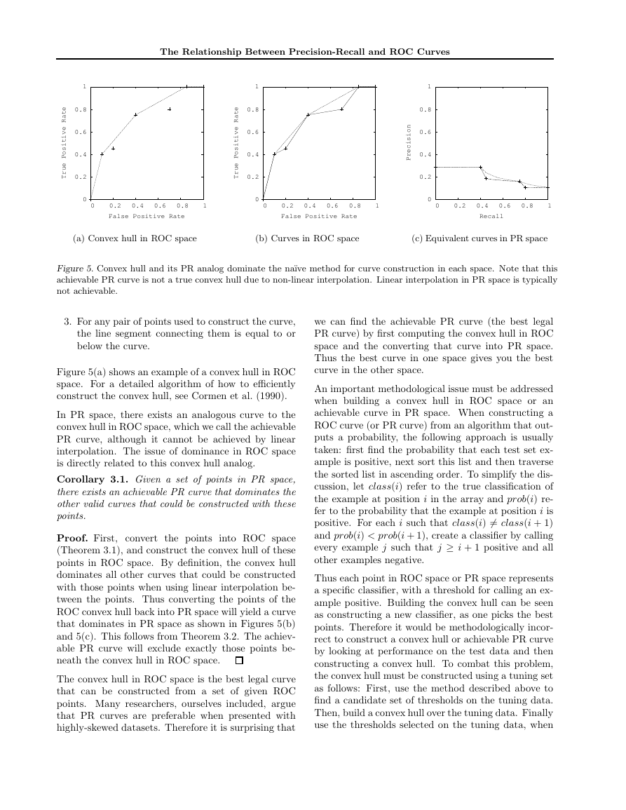
(a) Convex hull in ROC space
(b) Curves in ROC space
(c) Equivalent curves in PR space
Figure 5. Convex hull and its PR analog dominate the nave method for curve construction in each space. Note that this
achievable PR curve is not a true convex hull due to non-linear interpolation. Linear interpolation in PR space is typically
not achievable.
3. For any pair of points used to construct the curve,
the line segment connecting them is equal to or
below the curve.
Figure 5(a) shows an example of a convex hull in ROC
space. For a detailed algorithm of how to eciently
construct the convex hull, see Cormen et al. (1990).
In PR space, there exists an analogous curve to the
convex hull in ROC space, which we call the achievable
PR curve, although it cannot be achieved by linear
interpolation. The issue of dominance in ROC space
is directly related to this convex hull analog.
Corollary 3.1. Given a set of points in PR space,
there exists an achievable PR curve that dominates the
other valid curves that could be constructed with these
points.
Proof. First, convert the points into ROC space
(Theorem 3.1), and construct the convex hull of these
points in ROC space. By denition, the convex hull
dominates all other curves that could be constructed
with those points when using linear interpolation be-
tween the points. Thus converting the points of the
ROC convex hull back into PR space will yield a curve
that dominates in PR space as shown in Figures 5(b)
and 5(c). This follows from Theorem 3.2. The achiev-
able PR curve will exclude exactly those points be-
neath the convex hull in ROC space.
The convex hull in ROC space is the best legal curve
that can be constructed from a set of given ROC
points. Many researchers, ourselves included, argue
that PR curves are preferable when presented with
highly-skewed datasets. Therefore it is surprising that
we can nd the achievable PR curve (the best legal
PR curve) by rst computing the convex hull in ROC
space and the converting that curve into PR space.
Thus the best curve in one space gives you the best
curve in the other space.
An important methodological issue must be addressed
when building a convex hull
in ROC space or an
achievable curve in PR space. When constructing a
ROC curve (or PR curve) from an algorithm that out-
puts a probability, the following approach is usually
taken: rst nd the probability that each test set ex-
ample is positive, next sort this list and then traverse
the sorted list in ascending order. To simplify the dis-
cussion, let class(i) refer to the true classication of
the example at position i in the array and prob(i) re-
fer to the probability that the example at position i is
positive. For each i such that class(i) 6= class(i + 1)
and prob(i) < prob(i + 1), create a classier by calling
every example j such that j i + 1 positive and all
other examples negative.
Thus each point in ROC space or PR space represents
a specic classier, with a threshold for calling an ex-
ample positive. Building the convex hull can be seen
as constructing a new classier, as one picks the best
points. Therefore it would be methodologically incor-
rect to construct a convex hull or achievable PR curve
by looking at performance on the test data and then
constructing a convex hull. To combat this problem,
the convex hull must be constructed using a tuning set
as follows: First, use the method described above to
nd a candidate set of thresholds on the tuning data.
Then, build a convex hull over the tuning data. Finally
use the thresholds selected on the tuning data, when
�
The Relationship Between Precision-Recall and ROC Curves
building an ROC or PR curve for the test data. While
this test-data curve is not guaranteed to be a convex
hull, it preserves the split between training data and
testing data.
4. Interpolation and AUC
A key practical issue to address is how to interpolate
between points in each space.
It is straightforward
to interpolate between points in ROC space by sim-
ply drawing a straight line connecting the two points.
One can achieve any level of performance on this line
by ipping a weighted coin to decide between the clas-
siers that the two end points represent.
in Precision-Recall space,
However,
interpolation is
more complicated. As the level of Recall varies, the
Precision does not necessarily change linearly due to
the fact that F P replaces F N in the denominator of
the Precision metric. In these cases, linear interpola-
tion is a mistake that yields an overly-optimistic es-
timate of performance. Corollary 3.1 shows how to
nd the achievable PR curve by simply converting the
analogous ROC convex hull; this yields the correct in-
terpolation in PR space. However, a curve consists of
innitely many points, and thus we need a practical,
approximate method for translation. We expand here
on the method proposed by Goadrich et al. (2004) to
approximate the interpolation between two points in
PR space.
Remember that any point A in a Precision-Recall
space is generated from the underlying true positive
(T PA) and false positive (F PA) counts. Suppose we
have two points, A and B which are far apart in
Precision-Recall space. To nd some intermediate val-
ues, we must interpolate between their counts T PA
and T PB, and F PA and F PB. We nd out how many
negative examples it takes to equal one positive, or the
local skew, dened by F PB F PA
. Now we can create
T PB T PA
new points T PA +x for all integer values of x such that
1 x T PB T PA, i.e. T PA+1; T PA+2; :::; T PB 1,
and calculate corresponding FP by linearly increasing
the false positives for each new point by the local skew.
Our resulting intermediate Precision-Recall points will
be
T PA + x
Total Pos
;
T PA + x
T PA + x + F PA + F PB F PA
T PB T PA
x! :
For example, suppose we have a dataset with 20 posi-
tive examples and 2000 negative examples. Let T PA =
5, F PA = 5, T PB = 10, and F PB = 30. Table 1 shows
the proper interpolation of the intermediate points be-
tween A and B, with the local skew of 5 negatives for
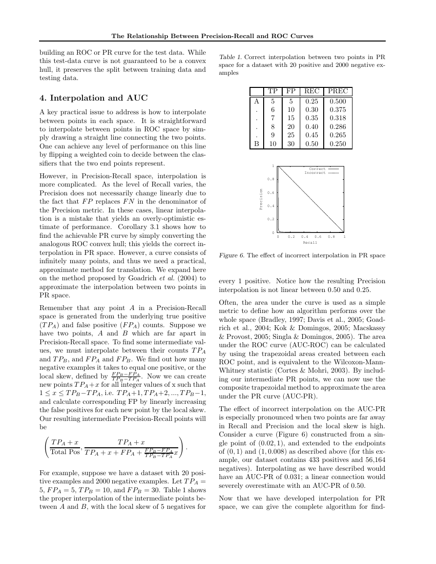
Table 1. Correct interpolation between two points in PR
space for a dataset with 20 positive and 2000 negative ex-
amples
TP FP REC PREC
0.500
5
0.375
6
0.318
7
8
0.286
0.265
9
10
0.250
0.25
0.30
0.35
0.40
0.45
0.50
5
10
15
20
25
30
A
.
.
.
.
B
1
0.8
n
o
i
s
i
c
e
r
P
0.6
0.4
0.2
0
Correct
Incorrect
0
0.2 0.4 0.6 0.8
1
Recall
Figure 6. The eect of incorrect interpolation in PR space
every 1 positive. Notice how the resulting Precision
interpolation is not linear between 0.50 and 0.25.
Often, the area under the curve is used as a simple
metric to dene how an algorithm performs over the
whole space (Bradley, 1997; Davis et al., 2005; Goad-
rich et al., 2004; Kok & Domingos, 2005; Macskassy
& Provost, 2005; Singla & Domingos, 2005). The area
under the ROC curve (AUC-ROC) can be calculated
by using the trapezoidal areas created between each
ROC point, and is equivalent to the Wilcoxon-Mann-
Whitney statistic (Cortes & Mohri, 2003). By includ-
ing our intermediate PR points, we can now use the
composite trapezoidal method to approximate the area
under the PR curve (AUC-PR).
The eect of incorrect interpolation on the AUC-PR
is especially pronounced when two points are far away
in Recall and Precision and the local skew is high.
Consider a curve (Figure 6) constructed from a sin-
gle point of (0:02; 1), and extended to the endpoints
of (0; 1) and (1; 0:008) as described above (for this ex-
ample, our dataset contains 433 positives and 56,164
negatives). Interpolating as we have described would
have an AUC-PR of 0.031; a linear connection would
severely overestimate with an AUC-PR of 0.50.
Now that we have developed interpolation for PR
space, we can give the complete algorithm for nd-
�
The Relationship Between Precision-Recall and ROC Curves
1
e
t
a
R
e
v
i
t
i
s
o
P
e
u
r
T
0.8
0.6
0.4
0.2
0
0
Curve I
Curve II
1
0.8
0.6
0.4
0.2
n
o
i
s
i
c
e
r
P
Curve I
Curve II
0.2 0.4 0.6 0.8
False Positive Rate
1
0
0
0.2
0.4
0.6
0.8
1
Recall
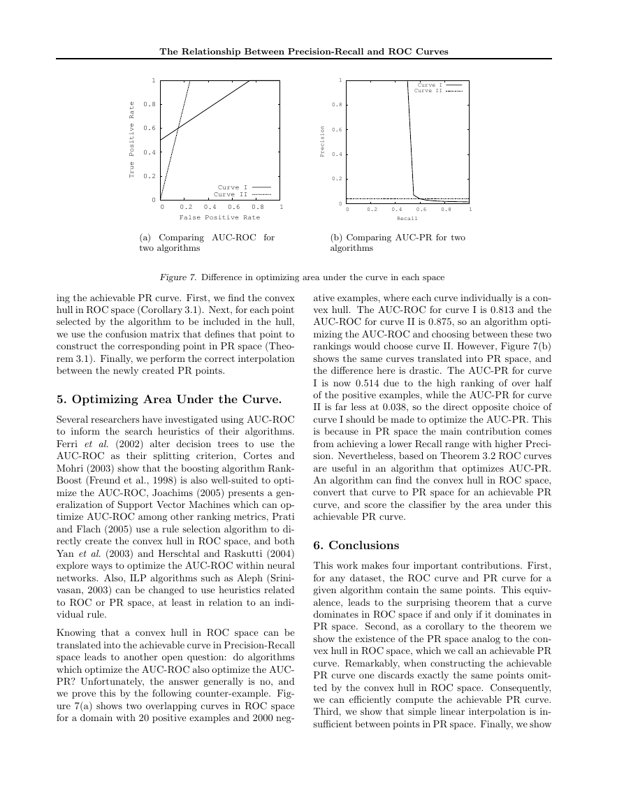
(a) Comparing AUC-ROC for
two algorithms
(b) Comparing AUC-PR for two
algorithms
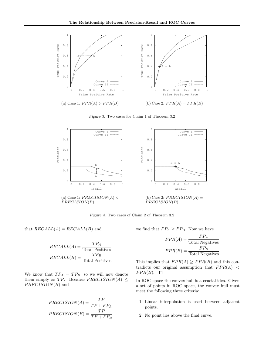
Figure 7. Dierence in optimizing area under the curve in each space
ing the achievable PR curve. First, we nd the convex
hull in ROC space (Corollary 3.1). Next, for each point
selected by the algorithm to be included in the hull,
we use the confusion matrix that denes that point to
construct the corresponding point in PR space (Theo-
rem 3.1). Finally, we perform the correct interpolation
between the newly created PR points.
5. Optimizing Area Under the Curve.
Several researchers have investigated using AUC-ROC
to inform the search heuristics of their algorithms.
Ferri et al. (2002) alter decision trees to use the
AUC-ROC as their splitting criterion, Cortes and
Mohri (2003) show that the boosting algorithm Rank-
Boost (Freund et al., 1998) is also well-suited to opti-
mize the AUC-ROC, Joachims (2005) presents a gen-
eralization of Support Vector Machines which can op-
timize AUC-ROC among other ranking metrics, Prati
and Flach (2005) use a rule selection algorithm to di-
rectly create the convex hull in ROC space, and both
Yan et al. (2003) and Herschtal and Raskutti (2004)
explore ways to optimize the AUC-ROC within neural
networks. Also, ILP algorithms such as Aleph (Srini-
vasan, 2003) can be changed to use heuristics related
to ROC or PR space, at least in relation to an indi-
vidual rule.
Knowing that a convex hull in ROC space can be
translated into the achievable curve in Precision-Recall
space leads to another open question: do algorithms
which optimize the AUC-ROC also optimize the AUC-
PR? Unfortunately, the answer generally is no, and
we prove this by the following counter-example. Fig-
ure 7(a) shows two overlapping curves in ROC space
for a domain with 20 positive examples and 2000 neg-
ative examples, where each curve individually is a con-
vex hull. The AUC-ROC for curve I is 0.813 and the
AUC-ROC for curve II is 0.875, so an algorithm opti-
mizing the AUC-ROC and choosing between these two
rankings would choose curve II. However, Figure 7(b)
shows the same curves translated into PR space, and
the dierence here is drastic. The AUC-PR for curve
I is now 0.514 due to the high ranking of over half
of the positive examples, while the AUC-PR for curve
II is far less at 0.038, so the direct opposite choice of
curve I should be made to optimize the AUC-PR. This
is because in PR space the main contribution comes
from achieving a lower Recall range with higher Preci-
sion. Nevertheless, based on Theorem 3.2 ROC curves
are useful in an algorithm that optimizes AUC-PR.
An algorithm can nd the convex hull in ROC space,
convert that curve to PR space for an achievable PR
curve, and score the classier by the area under this
achievable PR curve.
6. Conclusions
This work makes four important contributions. First,
for any dataset, the ROC curve and PR curve for a
given algorithm contain the same points. This equiv-
alence, leads to the surprising theorem that a curve
dominates in ROC space if and only if it dominates in
PR space. Second, as a corollary to the theorem we
show the existence of the PR space analog to the con-
vex hull in ROC space, which we call an achievable PR
curve. Remarkably, when constructing the achievable
PR curve one discards exactly the same points omit-
ted by the convex hull in ROC space. Consequently,
we can eciently compute the achievable PR curve.
Third, we show that simple linear interpolation is in-
sucient between points in PR space. Finally, we show
�
The Relationship Between Precision-Recall and ROC Curves
Goadrich, M., Oliphant, L., & Shavlik, J. (2004). Learn-
ing ensembles of rst-order clauses for recall-precision
curves: A case study in biomedical information extrac-
tion. Proceedings of the 14th International Conference
on Inductive Logic Programming (ILP). Porto, Portugal.
Herschtal, A., & Raskutti, B. (2004). Optimising area un-
der the ROC curve using gradient descent. Proceedings
of the 21st International Conference on Machine Learn-
ing (p. 49). New York, NY, USA: ACM Press.
Joachims, T. (2005). A support vector method for multi-
variate performance measures. Proceedings of the 22nd
International Conference on Machine Learning. ACM
Press.
Kok, S., & Domingos, P. (2005). Learning the structure of
Markov Logic Networks. Proceedings of 22nd Interna-
tional Conference on Machine Learning (pp. 441{448).
ACM Press.
Macskassy, S., & Provost, F. (2005). Suspicion scoring
based on guilt-by-association, collective inference, and
focused data access. International Conference on Intel-
ligence Analysis.
Manning, C., & Schutze, H. (1999). Foundations of statis-
tical natural language processing. MIT Press.
Prati, R., & Flach, P. (2005). ROCCER: an algorithm for
rule learning based on ROC analysis. Proceeding of the
19th International Joint Conference on Articial Intel-
ligence. Edinburgh, Scotland.
Provost, F., Fawcett, T., & Kohavi, R. (1998). The case
against accuracy estimation for comparing induction al-
gorithms. Proceeding of the 15th International Confer-
ence on Machine Learning (pp. 445{453). Morgan Kauf-
mann, San Francisco, CA.
Raghavan, V., Bollmann, P., & Jung, G. S. (1989). A
critical investigation of recall and precision as measures
of retrieval system performance. ACM Trans. Inf. Syst.,
7, 205{229.
Singla, P., & Domingos, P. (2005). Discriminative training
of Markov Logic Networks. Proceedings of the 20th Na-
tional Conference on Articial Intelligene (AAAI) (pp.
868{873). AAAI Press.
Srinivasan, A.
The Aleph Manual Version
4. http://web.comlab.ox.ac.uk/ oucl/ research/ areas/
machlearn/ Aleph/.
(2003).
Yan, L., Dodier, R., Mozer, M., & Wolniewicz, R. (2003).
Optimizing classier performance via the Wilcoxon-
Mann-Whitney statistics. Proceedings of the 20th In-
ternational Conference on Machine Learning.
that an algorithm that optimizes the area under the
ROC curve is not guaranteed to optimize the area un-
der the PR curve.
Acknowledgements
calculating
can
be
of
at
Java
all
found
program for
discussed metrics
A
the
http://www.cs.wisc.edu/~richm/programs/AUC/.
We gratefully acknowledge the funding from USA
NLM Grant 5T15LM007359-02 and USA Air Force
Grant F30602-01-2-0571, Vtor Santos Costa, Louis
Oliphant, our advisors David Page and Jude Shav-
lik and our anonymous reviewers for their helpful
comments and suggestions.
References
Bockhorst, J., & Craven, M. (2005). Markov networks for
detecting overlapping elements in sequence data. Neural
Information Processing Systems 17 (NIPS). MIT Press.
Bradley, A. (1997). The use of the area under the ROC
curve in the evaluation of machine learning algorithms.
Pattern Recognition, 30, 1145{1159.
Bunescu, R., Ge, R., Kate, R., Marcotte, E., Mooney, R.,
Ramani, A., & Wong, Y. (2004). Comparative Experi-
ments on Learning Information Extractors for Proteins
and their Interactions. Journal of Articial Intelligence
in Medicine, 139{155.
Cormen, T. H., Leiserson, Charles, E., & Rivest, R. L.
(1990). Introduction to algorithms. MIT Press.
Cortes, C., & Mohri, M. (2003). AUC optimization vs.
error rate minimization. Neural Information Processing
Systems 15 (NIPS). MIT Press.
Davis, J., Burnside, E., Dutra, I., Page, D., Ramakrishnan,
R., Costa, V. S., & Shavlik, J. (2005). View learning
for statistical relational learning: With an application
to mammography. Proceeding of the 19th International
Joint Conference on Articial Intelligence. Edinburgh,
Scotland.
Drummond, C., & Holte, R. (2000). Explicitly representing
expected cost: an alternative to ROC representation.
Proceeding of Knowledge Discovery and Datamining (pp.
198{207).
Drummond, C., & Holte, R. C. (2004). What ROC curves
can’t do (and cost curves can). ROCAI (pp. 19{26).
Ferri, C., Flach, P., & Henrandez-Orallo, J. (2002). Learn-
ing decision trees using area under the ROC curve. Pro-
ceedings of the 19th International Conference on Ma-
chine Learning (pp. 139{146). Morgan Kaufmann.
Freund, Y., Iyer, R., Schapire, R., & Singer, Y. (1998). An
ecient boosting algorithm for combining preferences.
Proceedings of the 15th International Conference on Ma-
chine Learning (pp. 170{178). Madison, US: Morgan
Kaufmann Publishers, San Francisco, US.
�


 2023年江西萍乡中考道德与法治真题及答案.doc
 2012年重庆南川中考生物真题及答案.doc
 2013年江西师范大学地理学综合及文艺理论基础考研真题.doc
 2020年四川甘孜小升初语文真题及答案I卷.doc
 2020年注册岩土工程师专业基础考试真题及答案.doc
 2023-2024学年福建省厦门市九年级上学期数学月考试题及答案.doc
 2021-2022学年辽宁省沈阳市大东区九年级上学期语文期末试题及答案.doc
 2022-2023学年北京东城区初三第一学期物理期末试卷及答案.doc
 2018上半年江西教师资格初中地理学科知识与教学能力真题及答案.doc
 2012年河北国家公务员申论考试真题及答案-省级.doc
 2020-2021学年江苏省扬州市江都区邵樊片九年级上学期数学第一次质量检测试题及答案.doc
 2022下半年黑龙江教师资格证中学综合素质真题及答案.doc