LDPC Codes: An Introduction
Amin Shokrollahi
Digital Fountain, Inc.
39141 Civic Center Drive, Fremont, CA 94538
amin@digitalfountain.com
April 2, 2003
Abstract
LDPC codes are one of the hottest topics in coding theory today. Originally invented in
the early 1960’s, they have experienced an amazing comeback in the last few years. Unlike
many other classes of codes LDPC codes are already equipped with very fast (probabilistic)
encoding and decoding algorithms. The question is that of the design of the codes such that these
algorithms can recover the original codeword in the face of large amounts of noise. New analytic
and combinatorial tools make it possible to solve the design problem. This makes LDPC codes
not only attractive from a theoretical point of view, but also perfect for practical applications. In
this note I will give a brief overview of the origins of LDPC codes and the methods used for their
analysis and design.
1
Introduction
This note constitutes an attempt to highlight some of the main aspects of the theory of low-density
parity-check (LDPC) codes. It is intended for a mathematically mature audience with some back-
ground in coding theory, but without much knowledge about LDPC codes.
The idea of writing a note like this came up during conversations that I had with Dr. Khos-
rovshahi, head of the Mathematics Section of the Institute for Studies in Theoretical Physics and
Mathematics in December 2002. The main motivation behind writing this note was to have a written
1
�
document for Master’s and PhD students who want to gain an understanding of LDPC codes at a
level where they feel comfortable deciding whether or not they want to pursue it as their research
topic. The style is often informal, though I have tried not to compromise exactness.
The note is by no means a survey. I have left out a number of interesting aspects of the theory,
such as connections to statistical mechanics, or articial intelligence. The important topics of general
Tanner graphs, and factor graphs have also been completely omitted. Connections to Turbo codes
have also been left untouched.
My emphasis in writing the notes has been on algorithmic and theoretical aspects of LDPC codes,
and within these areas on statements that can be proved. I have not discussed any of the existing and
very clever methods for the construction of LDPC codes, or issues regarding their implementation.
Nevertheless, I hope that this document proves useful to at least some students or researchers
interested in pursuing research in LDPC codes, or more generally codes obtained from graphs.
2 Shannon’s Theorem
The year 1948 marks the birth of information theory. In that year, Claude E. Shannon published his
epoch making paper [1] on the limits of reliable transmission of data over unreliable channels and
methods on how to achieve these limits. Among other things, this paper formalized the concept of
information, and established bounds for the maximum amount of information that can be transmitted
over unreliable channels.
A communication channel is usually dened as a triple consisting of an input alphabet, an out-
put alphabet, and for each pair (i; o) of input and output elements a transition probability p(i; o).
Semantically, the transition probability is the probability that the symbol o is received given that i
was transmitted over the channel.
Given a communication channel, Shannon proved that there exists a number, called the capacity
of the channel, such that reliable transmission is possible for rates arbitrarily close to the capacity,
and reliable transmission is not possible for rates above capacity.
The notion of capacity is dened purely in terms of information theory. As such it does not
guarantee the existence of transmission schemes that achieve the capacity. In the same paper Shannon
introduced the concept of codes as ensembles of vectors that are to be transmitted. In the following
I will try to motivate the concept.
It is clear that if the channel is such that even one input
2
�
element can be received in at least two possible ways (albeit with dierent probabilities), then
reliable communication over that channel is not possible if only single elements are sent over the
channel. This is the case even if multiple elements are sent that are not correlated (in a manner to
be made precise). To achieve reliable communication, it is thus imperative to send input elements
that are correlated. This leads to the concept of a code, dened as a (nite) set of vectors over the
input alphabet. We assume that all the vectors have the same length, and call this length the block
length of the code. If the number of vectors is K = 2k, then every vector can be described with k
bits. If the length of the vectors is n, then in n times use of the channel k bits have been transmitted.
We say then that the code has a rate of k=n bits per channel use, or k=n bpc.
Suppose now that we send a codeword, and receive a vector over the output alphabet. How do we
infer the vector that we sent? If the channel allows for errors, then there is no general way of telling
which codeword was sent with absolute certainty. However, we can nd the most likely codeword
that was sent, in the sense that the probability that this codeword was sent given the observed vector
is maximized. To see that we really can nd such a codeword, simply list all the K codewords, and
calculate the conditional probability for the individual codewords. Then nd the vector or vectors
that yield the maximum probability and return one of them. This decoder is called the maximum
likelihood decoder. It is not perfect: it takes a lot of time (especially when the code is large) and it
may err; but it is the best we can do.
Shannon proved the existence of codes of rates arbitrarily close to capacity for which the proba-
bility of error of the maximum likelihood decoder goes to zero as the block length of the code goes to
innity. (In fact, Shannon proved that the decoding error of the maximum likelihood decoder goes
to zero exponentially fast with the block length, but we will not discuss it here.)
Codes that approach capacity are very good from a communication point of view, but Shannon’s
theorems are non-constructive and don’t give a clue on how to nd such codes. More importantly,
even if an oracle gave us sequences of codes that achieve capacity for a certain rate, it is not clear
how to encode and decode them eciently. Design of codes with ecient encoding and decoding
algorithms which approach the capacity of the channel is the main topic of this note.
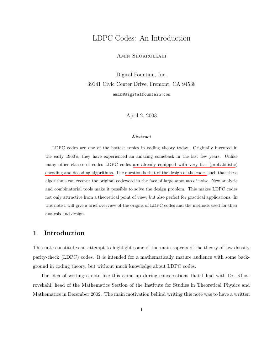
Before I close this section, let me give an example of two communication channels: the binary
erasure channel (BEC), and the binary symmetric channel (BSC). These channels are described in
Figure 1. In both cases the input alphabet is binary, and the elements of the input alphabet are
called bits.
In the case of the binary erasure channel the output alphabet consists of 0, 1, and
3
�
0
1
p
p
-p
1
-p
1
(a)
0
e
1
0
1
p
p
-p
1
-p
1
(b)
0
1
Figure 1: Two examples of channels: (a) The Binary Erasure Channel (BEC) with erasure probability
p, and (b) The Binary Symmetric Channel (BSC) with error probability p
an additional element denoted e and called erasure. Each bit is either transmitted correctly (with
probability 1 p), or it is erased (with probability p). The capacity of this channel is 1 p.
In the case of the BSC both the input and the output alphabet is F2. Each bit is either transmitted
correctly with probability 1 p, or it is ipped with probability p. This channel may seem simpler
than the BEC at rst sight, but in fact it is much more complicated. The complication arises since
it is not clear which bits are ipped. (In the case of the BEC it is clear which bits are erased.)
The capacity of this channel is 1 + p log2(p) + (1 p) log2(1 p). Maximum likelihood decoding for
this channel is equivalent to nding, for a given vector of length n over F2, a codeword that has
the smallest Hamming distance from the received word. It can be shown that maximum likelihood
decoding for the BSC is NP-complete [2]. In contrast, for linear codes maximum likelihood decoding
on the BEC is polynomial time, since it can be reduced to solving a system of equations (cf. [3]).
3 Algorithmic Issues
Soon after Shannon’s discoveries researchers found that random codes are capacity achieving.
In
fact, this is implicit in Shannon’s treatise itself.
But achieving capacity is only part of the story. If these codes are to be used for communication,
one needs fast algorithms for encoding and decoding. Note that random codes of rate R bpc are just
2Rn random vectors of length n over the input alphabet. We need some description of these vectors
to be able to embed information into them, or we need to write all of them down into a so-called
codebook describing which sequence of Rn bits gets mapped to which codeword. This requires a
4
�
codebook of size 2Rn, which is too big for any reasonably sized code (say of length 1000 and rate 0:5,
which yields 2500 vectors|too large to handle).
If the input alphabet has the structure of a eld (for example the binary alphabet which yields
the eld F2), then one can do better, at least as far as encoding goes. Elias and Golay independently
introduced the concept of linear codes of block length n and dimension k dened as subspaces of the
vector space Fn
2 . Such codes have rate k=n (we will omit the unit bpc for binary codes from now
on), and since they are linear, they can be described in terms of a basis consisting of k vectors of
length n. A codebook can now be implicitly described in a natural manner by mapping a bit vector
(x1; : : : ; xk) to the vector obtained by taking linear combinations of the basis vectors given by the
coecients x1; : : : ; xk.
The class of linear codes is very rich. Shannon’s arguments can be used (almost verbatim) to
show that there are sequences of linear codes with rates arbitrarily close to capacity and for which
the error probability of the maximum likelihood decoder approaches zero (exponentially fast) as
the block length goes to innity. Moreover, it can also be shown that random linear codes achieve
capacity. Unlike their non-linear brethren, linear codes can be encoded in polynomial time, rather
than exponential time. This is good news.
How about decoding? The decoding problem seems much tougher. As was mentioned above, the
maximum likelihood problem on the BSC has been shown to be NP-hard for many classes of linear
codes (e.g., general linear codes over Fq for any q). It is therefore unlikely to nd polynomial time
algorithms for maximum likelihood decoding of general linear codes. One way to get around this
negative result is to try to repeat the success story for the encoding problem and to specialize to
subclasses of general linear codes. However, we have not been able to nd subclasses of linear codes
for which maximum likelihood decoding is polynomial time and which achieve capacity.
Another possiblity is to look at sub-optimal algorithms that are polynomial time by construction.
This is the path we will follow in the next section.
4 LDPC Codes
LDPC codes were invented by Robert Gallager [4] in his PhD thesis. Soon after their invention, they
were largely forgotten, and reinvented several times for the next 30 years. Their comeback is one of
the most intriguing aspects of their history, since two dierent communities reinvented codes similar
5
�
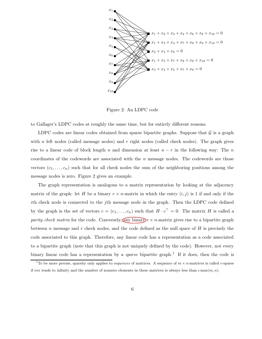
x1
x2
x3
x4
x5
x6
x7
x8
x9
x10
x1 + x2 + x3 + x4 + x6 + x8 + x10 = 0
x1 + x3 + x4 + x7 + x8 + x9 + x10 = 0
x2 + x4 + x8 = 0
x1 + x5 + x7 + x8 + x9 + x10 = 0
x3 + x4 + x5 + x7 + x9 = 0
Figure 2: An LDPC code
to Gallager’s LDPC codes at roughly the same time, but for entirely dierent reasons.
LDPC codes are linear codes obtained from sparse bipartite graphs. Suppose that G is a graph
with n left nodes (called message nodes) and r right nodes (called check nodes). The graph gives
rise to a linear code of block length n and dimension at least n r in the following way: The n
coordinates of the codewords are associated with the n message nodes. The codewords are those
vectors (c1; : : : ; cn) such that for all check nodes the sum of the neighboring positions among the
message nodes is zero. Figure 2 gives an example.
The graph representation is analogous to a matrix representation by looking at the adjacency
matrix of the graph: let H be a binary r n-matrix in which the entry (i; j) is 1 if and only if the
ith check node is connected to the jth message node in the graph. Then the LDPC code dened
by the graph is the set of vectors c = (c1; : : : ; cn) such that H c> = 0. The matrix H is called a
parity check matrix for the code. Conversely, any binary r n-matrix gives rise to a bipartite graph
between n message and r check nodes, and the code dened as the null space of H is precisely the
code associated to this graph. Therefore, any linear code has a representation as a code associated
to a bipartite graph (note that this graph is not uniquely dened by the code). However, not every
binary linear code has a representation by a sparse bipartite graph.1 If it does, then the code is
1To be more precise, sparsity only applies to sequences of matrices. A sequence of m n-matrices is called c-sparse
if mn tends to innity and the number of nonzero elements in these matrices is always less than c max(m; n).
6
�
called a low-density parity-check (LDPC) code.
The sparsity of the graph structure is key property that allows for the algorithmic eciency of
LDPC codes. The rest of this note is devoted to elaborating on this relationship.
5 Decoding Algorithms: Belief Propagation
Let me rst start by describing a general class of decoding algorithms for LDPC codes. These
algorithms are called message passing algorithms, and are iterative algorithms. The reason for their
name is that at each round of the algorithms messages are passed from message nodes to check nodes,
and from check nodes back to message nodes. The messages from message nodes to check nodes are
computed based on the observed value of the message node and some of the messages passed from
the neighboring check nodes to that message node. An important aspect is that the message that
is sent from a message node v to a check node c must not take into account the message sent in
the previous round from c to v. The same is true for messages passed from check nodes to message
nodes.
One important subclass of message passing algorithms is the belief propagation algorithm. This
algorithm is present in Gallager’s work [4], and it is also used in the Articial Intelligence commu-
nity [5]. The messages passed along the edges in this algorithm are probabilities, or beliefs. More
precisely, the message passed from a message node v to a check node c is the probability that v has
a certain value given the observed value of that message node, and all the values communicated to
v in the prior round from check nodes incident to v other than c. On the other hand, the message
passed from c to v is the probability that v has a certain value given all the messages passed to c in
the previous round from message nodes other than v.
It is easy to derive formulas for these probabilities under a certain assumption called independence
assumption, which I will discuss later. It is sometimes advantageous to work with likelihoods, or
sometimes even log-likelihoods instead of probabilities. For a binary random variable x let L(x) =
Pr[x = 0]=Pr[x = 1] be the likelihood of x. Given another random variable y, the conditional likelihood
of x denoted L(x j y) is dened as Pr[x = 0 j y]=Pr[x = 1 j y]. Similarly, the log-likelihood of x is
ln L(x), and the conditional log-likelihood of x given y is ln L(x j y).
If x is an equiprobable random variable, then L(x j y) = L(y j x) by Bayes’ rule. Therefore, if
7
�
y1; : : : ; yd are independent random variables, then we have
d
ln L(x j y1; : : : ; yd) =
ln L(x j yi):
(1)
Xi=1
Now suppose that x1; : : : ; x‘ are binary random variables and y1; : : : ; y‘ are random variables. Denote
addition over F2 by . We would like to calculate ln L(x1 x‘ j y1; : : : ; y‘). Note that if
p = 2Pr[x1 = 0 j y1] 1 and q = 2Pr[x2 = 0 j y2] 1, then 2Pr[x1 x2 = 0 j y1; y2] 1 = pq. (Why?)
Therefore, 2Pr[x1 x‘ = 0 j y1; : : : ; y‘] 1 =Q‘
L(xi j yi)=(1 + L(xi j yi)), we have that 2Pr[xi = 0 j yi] 1 = (L 1)=(L + 1) = tanh(‘=2), where
i=1(2Pr[xi = 0 j yi] 1). Since Pr[xi = 0 j yi] =
L = L(xi j yi) and ‘ = ln L. Therefore, we obtain
ln L(x1 x‘ j y1; : : : ; y‘) = ln
1 +Q‘
1 Q‘
i=1 tanh(‘i=2)
i=1 tanh(‘i=2)
;
(2)
where ‘i = ln L(xi j yi). The belief propagation algorithm for LDPC codes can be derived from
these two observations.
In round 0, the check nodes send along all the outgoing edges their log-
likelihoods conditioned on their observed value. For example, if the channel used is the BSC with
error probability p, then the rst message sent to all the check nodes adjacent to a message node
is ln(1 p) ln p if the node’s value is zero, and it is the negative of this value if the node’s value
is one. In all the subsequent rounds of the algorithm a check node c sends to an adjacent message
node v a likelihood according to (2). A message node v sends to the check node c its log-likelihood
conditioned on its observed value and on the incoming log-likelihoods from adjacent check nodes
other than c using the relation (1).
Let m
(‘)
vc be the message passed from message node v to check node c at the ‘th round of the
algorithm. Similarly, dene m
(‘)
cv . At round 0, m
(0)
vc is the log-likelihood of the message node v
conditioned on its observed value, which is independent of c. We denote this value by m v. Then the
update equations for the messages under belief-propagation can be described as
m(‘)
vc = 8<
:
m(‘)
cv = ln
mv;
mv +Pc
1 +Qv
1 Qv
02Cvnfcg m
(‘1)
0
c
v
;
if ‘ = 0;
if ‘ 1;
02Vcnfvg tanhm
02Vcnfvg tanhm
(‘)
0
v
(‘)
0
v
;
c=2
c=2
(3)
(4)
where Cv is the set of check nodes incident to message node v, and V c is the set of message nodes
incident to check node c.
8
�



 2023年江西萍乡中考道德与法治真题及答案.doc
 2012年重庆南川中考生物真题及答案.doc
 2013年江西师范大学地理学综合及文艺理论基础考研真题.doc
 2020年四川甘孜小升初语文真题及答案I卷.doc
 2020年注册岩土工程师专业基础考试真题及答案.doc
 2023-2024学年福建省厦门市九年级上学期数学月考试题及答案.doc
 2021-2022学年辽宁省沈阳市大东区九年级上学期语文期末试题及答案.doc
 2022-2023学年北京东城区初三第一学期物理期末试卷及答案.doc
 2018上半年江西教师资格初中地理学科知识与教学能力真题及答案.doc
 2012年河北国家公务员申论考试真题及答案-省级.doc
 2020-2021学年江苏省扬州市江都区邵樊片九年级上学期数学第一次质量检测试题及答案.doc
 2022下半年黑龙江教师资格证中学综合素质真题及答案.doc