See discussions, stats, and author profiles for this publication at: https://www.researchgate.net/publication/239523527
Empirical Wavelet Transform
Article in IEEE Transactions on Signal Processing · August 2013
DOI: 10.1109/TSP.2013.2265222
READS
1,334
CITATIONS
184
1 author:
Jerome Gilles
San Diego State University
36 PUBLICATIONS 496 CITATIONS
SEE PROFILE
Some of the authors of this publication are also working on these related projects:
Multicluster thresholding of unimodal histogram View project
Imaging Through Atmospheric Turbulence View project
All content following this page was uploaded by Jerome Gilles on 05 June 2014.
The user has requested enhancement of the downloaded file.
�
IEEE TRANS. ON SIGNAL PROCESSING, VOL. XX, NO. XX, FEBRUARY 2013
1
Empirical wavelet transform
J´erˆome Gilles
Abstract—Some recent methods, like the Empirical Mode De-
composition (EMD), propose to decompose a signal accordingly
to its contained information. Even though its adaptability seems
useful for many applications, the main issue with this approach
is its lack of theory. This paper presents a new approach to
build adaptive wavelets. The main idea is to extract the different
modes of a signal by designing an appropriate wavelet filter bank.
This construction leads us to a new wavelet transform, called the
empirical wavelet transform. Many experiments are presented
showing the usefulness of this method compared to the classic
EMD.
Index Terms—Wavelet, Empirical mode decomposition, Adap-
tive filtering
I. INTRODUCTION
A DAPTIVE methods to analyze a signal is of great in-
terest to find sparse representations in the context of
compressive sensing. “Rigid” methods, like the Fourier or
wavelets transforms, correspond to the use of some basis
(or frame) designed independently of the processed signal.
The aim of adaptive methods is to construct such a basis
directly based on the information contained in the signal.
A well known way to build an adaptive representations is
the basis pursuit approach which is used in the wavelet
packets transform. Even though the wavelet packets have
shown interesting results for practical applications, they still
are based on a prescribed subdivision scheme. A completely
different approach to build an adaptive representation is the
algorithm called “Empirical Mode Decomposition” (EMD)
proposed by Huang et al. [9]. The purpose of this method
is to detect the principal “modes” which represent the signal
(roughly speaking, a mode corresponds to a signal which have
a compactly supported Fourier spectrum). This method has
gained a lot of interest in signal analysis this last decade,
mainly because it
is able to separate stationary and non-
stationary components from a signal. However, the main issue
of the EMD approach is its lack of mathematical
theory.
Indeed, it is an algorithmic approach and, due to its non-
linearity, is difficult to model. Nevertheless, some experiments
[5]–[7] show that EMD behaves like an adaptive filter bank.
Some recent works attempt to model EMD in a variational
framework. In [4], the authors proposed to model a mode
as an amplitude modulated-frequency modulated (AM-FM)
Manuscript received October, 2012. Revised version received February,
2013. Copyright (c) 2012 IEEE. Personal use of this material is permitted.
However, permission to use this material for any other purposes must be
obtained from the IEEE by sending a request to pubs-permissions@ieee.org
J. Gilles is with the Department of Mathematics, University of California,
Los Angeles (UCLA), 520 Portola Plaza, Los Angeles, CA 90024, USA email:
jegilles@math.ucla.edu.
This work was partially founded by the following grants NSF DMS-
0914856, NSF DMS-1118971, ONR N00014-08-1-1119, ONR N0014-09-1-
0360, ONR MURI USC, the UC Lab Fees Research and the Keck Foundation.
signal and then use the properties of such signals to build
a functional to represent the whole signal. Then they are able
to retrieve the different modes by minimizing this functional.
Another proposed variational approach is the work of Hou
et al. [8] where the authors also use the AM-FM formalism.
They propose to minimize a functional which is build on
some regularity assumptions about the different components
and uses higher-order total variation priors.
In this paper, we propose a new approach to build adaptive
wavelets capable of extracting AM-FM components of a
signal. The key idea is that such AM-FM components have
a compact support Fourier spectrum. Separating the different
modes is equivalent to segment the Fourier spectrum and to
apply some filtering corresponding to each detected support.
We will show that it is possible to adapt the wavelet formalism
by considering distinct Fourier supports and then build a set
of functions which form an orthonormal basis. Based on this
construction, we propose an empirical wavelet transform (and
its inverse) to analyze a signal.
The remainder of the paper is organized as follows. Section II
has two distinct subsections: in II-A, we recall the principle
of the EMD algorithm and the AM-FM model; while in II-B,
we recall some wavelet formalism which will be useful in
our own construction and we discuss some of the existing
adaptive wavelet methods. In section III, we build the proposed
empirical wavelets and give some of their properties, then the
empirical wavelet transform and its inverse are introduced.
Section IV show many experiments based on simulated and
real signals. The time-frequency representation based on the
Hilbert transform is introduced in section V. In section VI,
we address the question of the estimation of the number of
modes. An extension to 2D signals (images) is presented in
section VII. Finally, we conclude and give some perspectives
in section VIII.
II. EXISTING APPROACHES
A. Empirical Mode Decomposition
In 1998, Huang et al. [9] proposed an original method
called Empirical Mode Decomposition (EMD) to decompose
a signal
into specific modes (we define the meaning of
“mode” hereafter). Its particularity is that it does not use any
prescribed function basis but it is self adapting accordingly
to the analyzed signal f (t). In this paper, as we will use the
Fourier formalism in section III, we adopt the description used
in [4] which is slightly different from the original used in [9].
EMD aims to decompose a signal as a (finite) sum of N + 1
Intrinsic Mode Functions (IMF) fk(t) such that
N
k=0
f (t) =
fk(t).
(1)
�
2
IEEE TRANS. ON SIGNAL PROCESSING, VOL. XX, NO. XX, FEBRUARY 2013
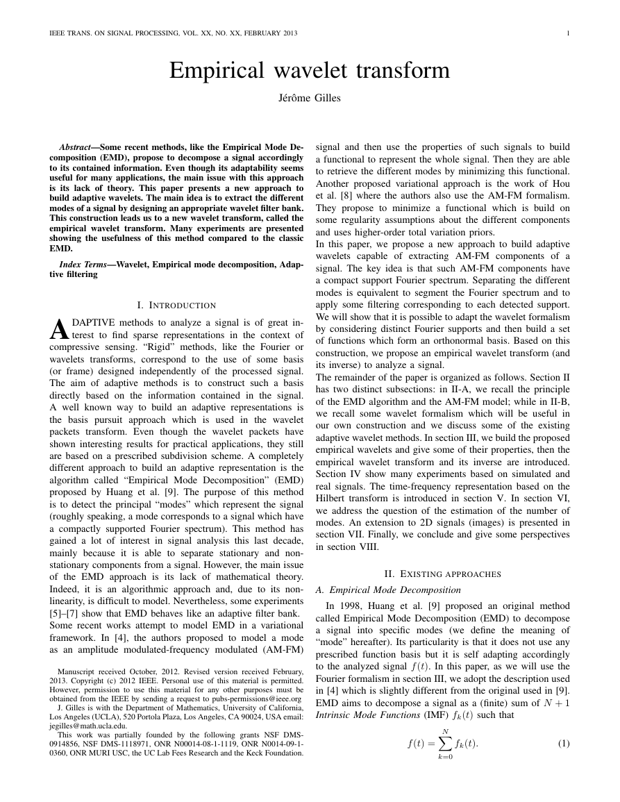
Fig. 1.
EMD: basic IMF detection. Envelopes detection on top (thin
continuous: f, dashed: ¯f and f and thick continuous: m). On bottom: the
first IMF candidate r1.
An IMF is an amplitude modulated-frequency modulated
function which can be written in the form
where Fk(t), ϕ
k(t) > 0 ∀t.
fk(t) = Fk(t) cos (ϕk(t))
(2)
The main assumption is that Fk and ϕ
k vary much slower
than ϕk. The IMF fk behaves as a harmonic component.
Originally, the method of Huang et al. [9] to extract such
IMFs is a pure algorithmic method. Candidates for an IMF are
extracted by first computing the upper, ¯f (t), and lower, f (t),
envelopes via a cubic spline interpolation from the maxima
and minima of f. Then the mean envelope is obtained by
computing m(t) = ( ¯f (t) + f (t))/2 and finally the candidate
by r1(t) = f (t) − m(t) (see Fig. 1). Generally, r1(t) does
not fulfill the properties of an IMF. A good candidate can be
reached by iterating the same process to r1 and the subsequent
rk. The final retained IMF is f1(t) = rn(t). Then the next IMF
is obtained by the same algorithm applied on f (t)−f1(t). The
remaining IMFs can be computed by repeating this algorithm
on the successive residues.
The interesting fact about this algorithm is that it is highly
adaptable and is able to extract the non-stationary part of
the original function. However, its main problem is that it is
based on an ad-hoc process which is mathematically difficult
to model. Consequently it is difficult to really understand
what the EMD provides. For example, some problems appear
when some noise is present in the signal. To deal with this
problem, an Ensemble EMD (EEMD) was proposed in [17].
The authors propose to compute several EMD decompositions
of the original signal corrupted by different artificial noises.
Then the final EEMD is the average of each EMD. This
approach seems to stabilize the obtained decomposition but
it increases the computational cost.
Another EMD approach is proposed in [8]. The authors
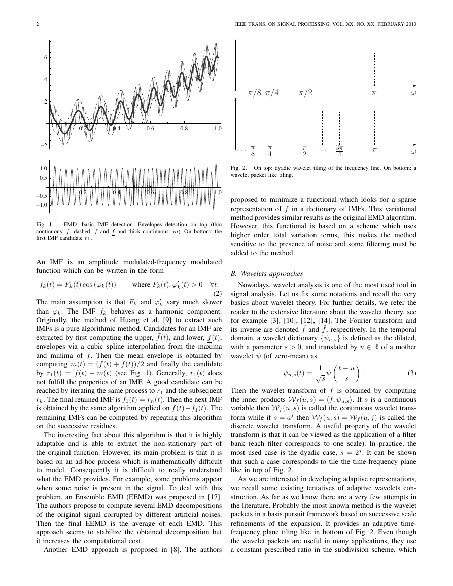
Fig. 2. On top: dyadic wavelet tiling of the frequency line. On bottom: a
wavelet packet like tiling.
proposed to minimize a functional which looks for a sparse
representation of f in a dictionary of IMFs. This variational
method provides similar results as the original EMD algorithm.
However, this functional is based on a scheme which uses
higher order total variation terms,
this makes the method
sensitive to the presence of noise and some filtering must be
added to the method.
B. Wavelets approaches
Nowadays, wavelet analysis is one of the most used tool in
signal analysis. Let us fix some notations and recall the very
basics about wavelet theory. For further details, we refer the
reader to the extensive literature about the wavelet theory, see
for example [3], [10], [12], [14]. The Fourier transform and
its inverse are denoted ˆf and ˇf, respectively. In the temporal
domain, a wavelet dictionary {ψu,s} is defined as the dilated,
with a parameter s > 0, and translated by u ∈ R of a mother
wavelet ψ (of zero-mean) as
t − u
ψu,s(t) =
1
√s
ψ
s
.
(3)
Then the wavelet transform of f is obtained by computing
the inner products Wf (u, s) = f, ψu,s. If s is a continuous
variable then Wf (u, s) is called the continuous wavelet trans-
form while if s = aj then Wf (u, s) = Wf (u, j) is called the
discrete wavelet transform. A useful property of the wavelet
transform is that it can be viewed as the application of a filter
bank (each filter corresponds to one scale). In practice, the
most used case is the dyadic case, s = 2j. It can be shown
that such a case corresponds to tile the time-frequency plane
like in top of Fig. 2.
As we are interested in developing adaptive representations,
we recall some existing tentatives of adaptive wavelets con-
struction. As far as we know there are a very few attempts in
the literature. Probably the most known method is the wavelet
packets in a basis pursuit framework based on successive scale
refinements of the expansion. It provides an adaptive time-
frequency plane tiling like in bottom of Fig. 2. Even though
the wavelet packets are useful in many applications, they use
a constant prescribed ratio in the subdivision scheme, which
0.20.40.60.81.0-22460.20.40.60.81.0-1.0-0.50.51.0ωππ/2π/4π/8...ωππ2π4π83π4......�
GILLES: EMPIRICAL WAVELET TRANSFORM
3
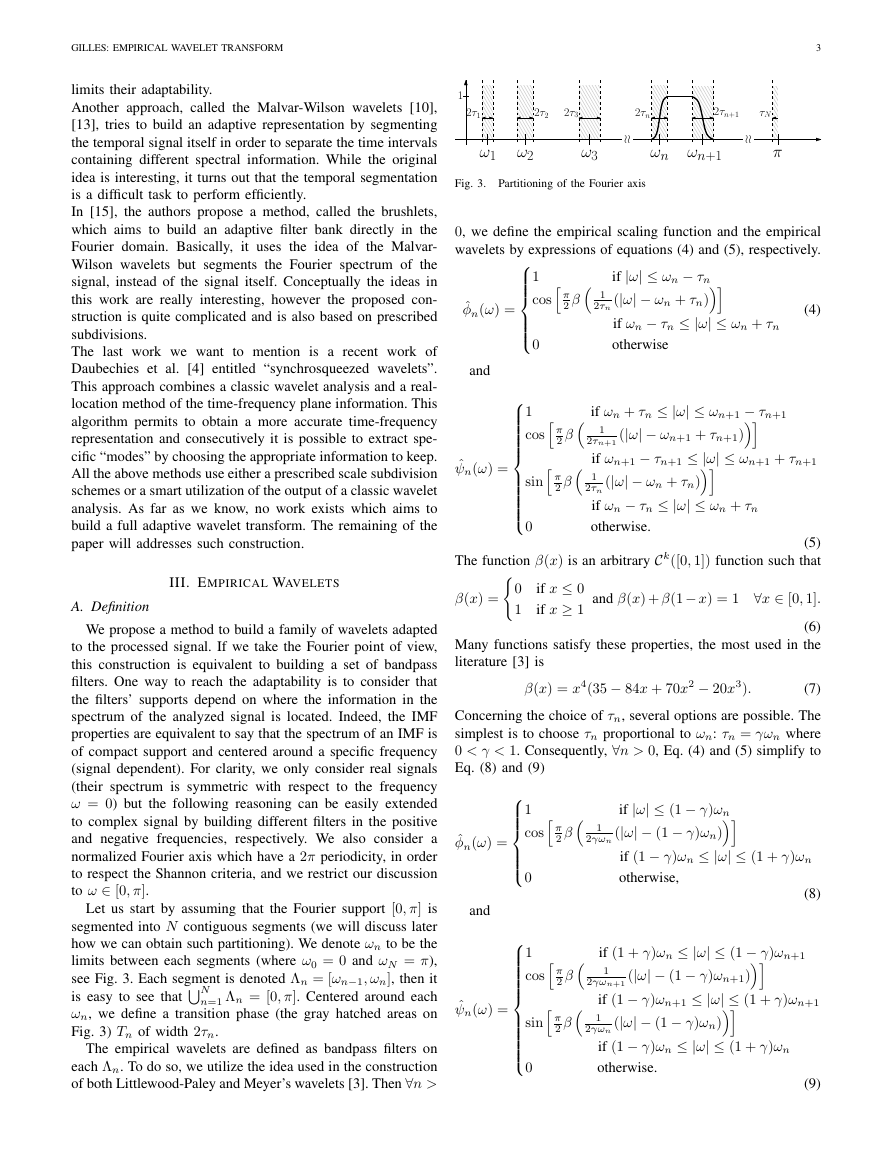
Fig. 3. Partitioning of the Fourier axis
limits their adaptability.
Another approach, called the Malvar-Wilson wavelets [10],
[13], tries to build an adaptive representation by segmenting
the temporal signal itself in order to separate the time intervals
containing different spectral information. While the original
idea is interesting, it turns out that the temporal segmentation
is a difficult task to perform efficiently.
In [15], the authors propose a method, called the brushlets,
which aims to build an adaptive filter bank directly in the
Fourier domain. Basically, it uses the idea of the Malvar-
Wilson wavelets but segments the Fourier spectrum of the
signal, instead of the signal itself. Conceptually the ideas in
this work are really interesting, however the proposed con-
struction is quite complicated and is also based on prescribed
subdivisions.
The last work we want
to mention is a recent work of
Daubechies et al. [4] entitled “synchrosqueezed wavelets”.
This approach combines a classic wavelet analysis and a real-
location method of the time-frequency plane information. This
algorithm permits to obtain a more accurate time-frequency
representation and consecutively it is possible to extract spe-
cific “modes” by choosing the appropriate information to keep.
All the above methods use either a prescribed scale subdivision
schemes or a smart utilization of the output of a classic wavelet
analysis. As far as we know, no work exists which aims to
build a full adaptive wavelet transform. The remaining of the
paper will addresses such construction.
III. EMPIRICAL WAVELETS
A. Definition
We propose a method to build a family of wavelets adapted
to the processed signal. If we take the Fourier point of view,
this construction is equivalent to building a set of bandpass
filters. One way to reach the adaptability is to consider that
the filters’ supports depend on where the information in the
spectrum of the analyzed signal is located. Indeed, the IMF
properties are equivalent to say that the spectrum of an IMF is
of compact support and centered around a specific frequency
(signal dependent). For clarity, we only consider real signals
(their spectrum is symmetric with respect to the frequency
ω = 0) but the following reasoning can be easily extended
to complex signal by building different filters in the positive
and negative frequencies, respectively. We also consider a
normalized Fourier axis which have a 2π periodicity, in order
to respect the Shannon criteria, and we restrict our discussion
to ω ∈ [0, π].
Let us start by assuming that the Fourier support [0, π] is
segmented into N contiguous segments (we will discuss later
how we can obtain such partitioning). We denote ωn to be the
limits between each segments (where ω0 = 0 and ωN = π),
see Fig. 3. Each segment is denoted Λn = [ωn−1, ωn], then it
n=1 Λn = [0, π]. Centered around each
ωn, we define a transition phase (the gray hatched areas on
Fig. 3) Tn of width 2τn.
is easy to see that N
The empirical wavelets are defined as bandpass filters on
each Λn. To do so, we utilize the idea used in the construction
of both Littlewood-Paley and Meyer’s wavelets [3]. Then ∀n >
1
0
1
0
1
0
ˆφn(ω) =
and
ˆψn(ω) =
0, we define the empirical scaling function and the empirical
wavelets by expressions of equations (4) and (5), respectively.
π
1
2 β
2τn
if |ω| ≤ ωn − τn
(|ω| − ωn + τn)
if ωn − τn ≤ |ω| ≤ ωn + τn
otherwise
1
cos
0
(4)
π
π
1
1
2τn
cos
2 β
sin
2 β
if ωn + τn ≤ |ω| ≤ ωn+1 − τn+1
2τn+1
(|ω| − ωn+1 + τn+1)
if ωn+1 − τn+1 ≤ |ω| ≤ ωn+1 + τn+1
(|ω| − ωn + τn)
if ωn − τn ≤ |ω| ≤ ωn + τn
otherwise.
(5)
The function β(x) is an arbitrary Ck([0, 1]) function such that
and β(x) + β(1− x) = 1 ∀x ∈ [0, 1].
β(x) =
(6)
Many functions satisfy these properties, the most used in the
literature [3] is
if x ≤ 0
if x ≥ 1
0
1
β(x) = x4(35 − 84x + 70x2 − 20x3).
(7)
Concerning the choice of τn, several options are possible. The
simplest is to choose τn proportional to ωn: τn = γωn where
0 < γ < 1. Consequently, ∀n > 0, Eq. (4) and (5) simplify to
Eq. (8) and (9)
ˆφn(ω) =
and
ˆψn(ω) =
π
1
cos
2 β
2γωn
if |ω| ≤ (1 − γ)ωn
(|ω| − (1 − γ)ωn)
if (1 − γ)ωn ≤ |ω| ≤ (1 + γ)ωn
otherwise,
(8)
π
π
1
if (1 + γ)ωn ≤ |ω| ≤ (1 − γ)ωn+1
cos
2 β
1
2γωn+1
(|ω| − (1 − γ)ωn+1)
if (1 − γ)ωn+1 ≤ |ω| ≤ (1 + γ)ωn+1
sin
2 β
2γωn
(|ω| − (1 − γ)ωn)
if (1 − γ)ωn ≤ |ω| ≤ (1 + γ)ωn
otherwise.
(9)
πω1ω2ω3ωnωn+1oo2τ12τ22τ32τn2τn+1τN1oo�
4
IEEE TRANS. ON SIGNAL PROCESSING, VOL. XX, NO. XX, FEBRUARY 2013
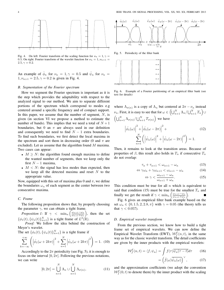
Fig. 4. On left: Fourier transform of the scaling function for νn = 1, γ =
0.5. On right: Fourier transform of the wavelet function for νn = 1, νn+1 =
2.5, γ = 0.2.
An example of ˆφn for νn = 1, γ = 0.5 and ˆψn for νn =
1, νn+1 = 2.5, γ = 0.2 is given in Fig. 4.
B. Segmentation of the Fourier spectrum
How we segment the Fourier spectrum is important as it is
the step which provides the adaptability with respect to the
analyzed signal to our method. We aim to separate different
portions of the spectrum which correspond to modes e.g
centered around a specific frequency and of compact support.
In this paper, we assume that the number of segment, N, is
given (in section VI we propose a method to estimate the
number of bands). This implies that we need a total of N + 1
boundaries, but 0 an π are always used in our definition
and consequently we need to find N − 1 extra boundaries.
To find such boundaries, we first detect the local maxima in
the spectrum and sort them in decreasing order (0 and π are
excluded). Let us assume that the algorithm found M maxima.
Two cases can appear:
• M ≥ N: the algorithm found enough maxima to define
the wanted number of segments, then we keep only the
first N − 1 maxima,
• M < N: the signal has less modes than expected, then
we keep all the detected maxima and reset N to the
appropriate value.
Now, equipped with this set of maxima plus 0 and π, we define
the boundaries ωn of each segment as the center between two
consecutive maxima.
C. Frame
The following proposition shows that, by properly choosing
the parameter γ, we can obtain a tight frame.
Proposition 1: If γ < minn
then the set
ωn+1−ωn
,
n=1} is a tight frame of L2(R).
ωn+1+ωn
Proof: We follow the idea behind the construction of
{φ1(t),{ψn(t)}N
Meyer’s wavelet.
+∞
The set {φ1(t),{ψn(t)}N
ˆφ1(ω + 2kπ)
2
Fig. 5. Periodicity of the filter bank
Fig. 6.
text for details)
Example of a Fourier partitioning of an empirical filter bank (see
where Λσ(n) is a copy of Λn but centered at 2π − νn instead
νn. First, it is easy to see that for ω ∈
∪
we have
N
n+1 Λn/N
ˆφ1(ω − 2π)
2
ˆψn(ω)
2
ˆψn(ω − 2π)
2
N
n=1 Λσ(n)/N
2
ˆφ1(ω)
N
n+1 Tσ(n)
n+1 Tn
(12)
= 1.
+
+
+
n=1
Then, it remains to look at the transition areas. Because of
properties of β, this result also holds in Tn if consecutive Tn
do not overlap:
τn + τn+1 < ωn+1 − ωn
⇔ γωn + γωn+1 < ωn+1 − ωn
⇔ γ <
ωn+1 − ωn
ωn+1 + ωn
.
(13)
(14)
(15)
This condition must be true for all n which is equivalent to
said that condition (15) must be true for the smallest Tn and
finally we get the result if γ < minn
.
ωn+1−ωn
Fig. 6 gives an empirical filter bank example based on the
set ωn ∈ {0, 1.5, 2, 2.8, π} with γ = 0.05 (the theory tells us
that γ < 0.057).
ωn+1+ωn
D. Empirical wavelet transform
N
n=1} is a tight frame if
+
ˆψn(ω + 2kπ)
2
= 1. (10)
From the previous section, we know how to build a tight
frame set of empirical wavelets. We can now define the
E
f (n, t), in the same
Empirical Wavelet Transform (EWT), W
way as for the classic wavelet transform. The detail coefficients
are given by the inner products with the empirical wavelets:
W
E
f (n, t) = f, ψn =
=
ˆf (ω) ˆψn(ω)
∨
f (τ )ψn(τ − t)dτ
,
(16)
(17)
k=−∞
Accordingly to the 2π periodicity (see Fig. 5), it is enough to
focus on the interval [0, 2π]. Following the previous notations,
we can write
n=1
N
N
[0, 2π] =
Λn ∪
n=1
n=1
Λσ(n),
(11)
and the approximation coefficients (we adopt the convention
E
f (0, t) to denote them) by the inner product with the scaling
W
-Π-Π2-101Π2Π0.20.40.60.81.0-Π-Π2-101Π2Π0.20.40.60.81.0ωNωN−1ω1ω2=π2π1ˆφ1(ω)ˆψ1(ω)ˆψN(ω)ˆψN(ω−2π)ˆψ1(ω−2π)ˆφ1(ω−2π)oooo-3-2-11230.20.40.60.81.0�
GILLES: EMPIRICAL WAVELET TRANSFORM
5
function:
W
E
f (0, t) = f, φ1 =
=
ˆf (ω) ˆφ1(ω)
∨
,
f (τ )φ1(τ − t)dτ
(18)
(19)
where ˆψn(ω) and ˆφ1(ω) are defined by Eq. 9 and 8, respec-
tively. The reconstruction is obtained by
f (t) = W
W
E
f (0, t) φ1(t) +
E
f (n, t) ψn(t)
=
E
f (0, ω) ˆφ1(ω) +
E
f (n, ω) ˆψn(ω)
∨
(20)
.
(21)
N
N
n=1
n=1
W
W
Following this formalism, the empirical mode fk, as defined
in section II-A, is given by
f0(t) = W
fk(t) = W
E
f (0, t) φ1(t),
E
f (k, t) ψk(t).
IV. EXPERIMENTS
(22)
(23)
A. Test signals
We propose to test the Empirical Wavelet Transform on four
different signals: three are artificial signals taken from [8] and
one real electrocardiogram signal. Their description is given
hereafter.
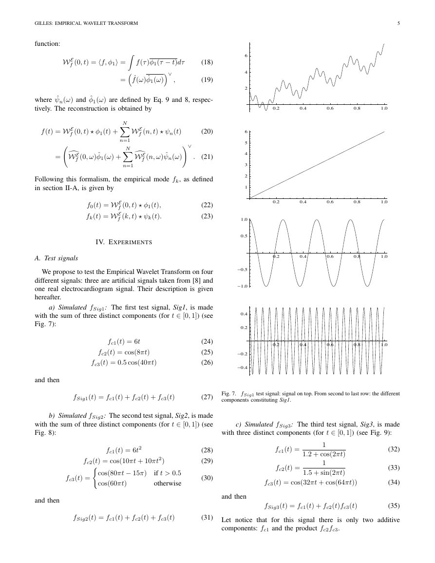
a) Simulated fSig1: The first test signal, Sig1, is made
with the sum of three distinct components (for t ∈ [0, 1]) (see
Fig. 7):
fc1(t) = 6t
fc2(t) = cos(8πt)
fc3(t) = 0.5 cos(40πt)
(24)
(25)
(26)
and then
fSig1(t) = fc1(t) + fc2(t) + fc3(t)
(27)
Fig. 7. fSig1 test signal: signal on top. From second to last row: the different
components constituting Sig1.
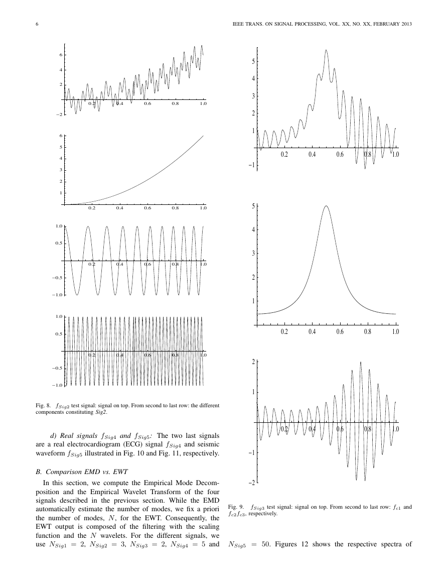
b) Simulated fSig2: The second test signal, Sig2, is made
with the sum of three distinct components (for t ∈ [0, 1]) (see
Fig. 8):
fc1(t) = 6t2
fc2(t) = cos(10πt + 10πt2)
cos(80πt − 15π)
cos(60πt)
if t > 0.5
otherwise
fc3(t) =
and then
fSig2(t) = fc1(t) + fc2(t) + fc3(t)
(28)
(29)
(30)
(31)
c) Simulated fSig3: The third test signal, Sig3, is made
with three distinct components (for t ∈ [0, 1]) (see Fig. 9):
fc1(t) =
fc2(t) =
1
1.2 + cos(2πt)
1
1.5 + sin(2πt)
(32)
(33)
(34)
(35)
and then
fc3(t) = cos(32πt + cos(64πt))
fSig3(t) = fc1(t) + fc2(t)fc3(t)
Let notice that for this signal
components: fc1 and the product fc2fc3.
there is only two additive
0.20.40.60.81.02460.20.40.60.81.01234560.20.40.60.81.0-1.0-0.50.51.00.20.40.60.81.0-0.4-0.20.20.4�
6
IEEE TRANS. ON SIGNAL PROCESSING, VOL. XX, NO. XX, FEBRUARY 2013
Fig. 8. fSig2 test signal: signal on top. From second to last row: the different
components constituting Sig2.
d) Real signals fSig4 and fSig5: The two last signals
are a real electrocardiogram (ECG) signal fSig4 and seismic
waveform fSig5 illustrated in Fig. 10 and Fig. 11, respectively.
B. Comparison EMD vs. EWT
In this section, we compute the Empirical Mode Decom-
position and the Empirical Wavelet Transform of the four
signals described in the previous section. While the EMD
automatically estimate the number of modes, we fix a priori
the number of modes, N, for the EWT. Consequently, the
EWT output is composed of the filtering with the scaling
function and the N wavelets. For the different signals, we
use NSig1 = 2, NSig2 = 3, NSig3 = 2, NSig4 = 5 and
Fig. 9.
fc2fc3, respectively.
fSig3 test signal: signal on top. From second to last row: fc1 and
NSig5 = 50. Figures 12 shows the respective spectra of
0.20.40.60.81.0-22460.20.40.60.81.01234560.20.40.60.81.0-1.0-0.50.51.00.20.40.60.81.0-1.0-0.50.51.00.20.40.60.81.0-1123450.20.40.60.81.0123450.20.40.60.81.0-2-112�
GILLES: EMPIRICAL WAVELET TRANSFORM
7
Fig. 10.
fSig4: real ECG signal.
Fig. 11.
fSig5: real seismic waveform signal.
Fig. 12. Detected Fourier supports for signals fSig1 to fSig4.
each test signal and the detected boundaries for each filter
support. We can observe that the algorithm is able is isolate the
E
different modes. The corresponding filtered signals W
f (n, t)
are presented in Fig. 13, 14, 15 and 17; while the EMD outputs
are given in Fig. 18, 19, 20 and 21, respectively.
We can observe that for the simulated test signals, the EMD
always overestimates the number of modes and then sepa-
rate some information which is originally part of the same
component. Except for the high frequencies, it is difficult
to interpret
the EMD outputs compared with the known
“true” components constituting the test signals. Concerning
the results given by the EWT, we can see that it is able to
detect the presence of modes in the spectrum and provides
different components which are close to the original ones.
However, in the case of fSig2, we can note that the algorithm
separates the two last modes which were initially parts of the
same component. In fact, this is not completely surprising
as those modes have significant individual energy and can
be considered as independent modes. About fSig3, another
phenomenon appears. The initial part fc1 is decomposed as
the sum of two modes (this sum is given in Fig. 16). If we
look more closely, the detected boundaries, shown in Fig. 12,
we can see that the scaling function is built upon a very small
support while the next support contains the main information
of fc1. If we ask the EWT to consider only N = 1 (as it
supposed to be from the construction of fSig3), the first two
supports shown in Fig. 12 are merged except that its boundary
is moved closer to the zero frequency. This change in the
boundary position has the consequence that some information
of fc1 is now on the second support and then appear in the
second mode instead the first one. In some sense, if we ask
to use N = 1, we get a perturbed decomposition. This issue
comes from the method we use to detect the boundaries of the
Fourier support and suggests more investigations.
Experiments on the real ECG signal seem to give the ad-
vantage to the EWT because the EMD provides too many
modes. Typically,
the EMD modes six to nine are really
difficult to interpret as such behavior is clearly not visible
the EWT focuses on the
in the signal
itself. A contrary,
Fig. 13. Modes extracted by the Empirical Wavelet Transform for fSig1.
oscillating patterns we can observe in fSig4. Of course it will
be very interesting to have the opinion of a cardiologist about
the medical interpretation of such components. The different
modes for the seismic signal are not provided here but we
will present its time-frequency representation in section V as
it more relevant for analysis purposes.
V. TIME-FREQUENCY REPRESENTATION
The time-frequency representation is useful
to have the
information of all components summarized in a single domain.
In this paper, we follow the idea used in the Hilbert-Huang
transform [9]. First, let us recall the definition of the Hilbert
transform of a function f:
+∞
−∞
f (τ )
t − τ
Hf (t) =
1
π
p.v.
dτ
(36)
where the integral is defined by using the Cauchy principal
value (p.v.) [11]. The Hilbert transform can be used to derive
1000200030004000-0.20.20.40.6200040006000800010000100050050010000.050.100.151000200030004000500060000.20.40.60.81000200030004000ˆfSig1ˆfSig20.050.100.150.200.250.30500100015002000250030000.020.040.060.080.100.120.1450100150200250ˆfSig3ˆfSig40.20.40.60.81.01234560.20.40.60.81.0-1.0-0.50.51.00.20.40.60.81.0-0.4-0.20.20.40.6�



 2023年江西萍乡中考道德与法治真题及答案.doc
 2012年重庆南川中考生物真题及答案.doc
 2013年江西师范大学地理学综合及文艺理论基础考研真题.doc
 2020年四川甘孜小升初语文真题及答案I卷.doc
 2020年注册岩土工程师专业基础考试真题及答案.doc
 2023-2024学年福建省厦门市九年级上学期数学月考试题及答案.doc
 2021-2022学年辽宁省沈阳市大东区九年级上学期语文期末试题及答案.doc
 2022-2023学年北京东城区初三第一学期物理期末试卷及答案.doc
 2018上半年江西教师资格初中地理学科知识与教学能力真题及答案.doc
 2012年河北国家公务员申论考试真题及答案-省级.doc
 2020-2021学年江苏省扬州市江都区邵樊片九年级上学期数学第一次质量检测试题及答案.doc
 2022下半年黑龙江教师资格证中学综合素质真题及答案.doc