Model Free Adaptive Control with Disturbance Observer.pdf-资料库

CEAI, Vol.14, No.4, pp. 42-49, 2012 Printed in Romania Model Free Adaptive Control with Disturbance Observer Bu Xuhui*, Hou Zhongsheng**, Yu Fashan*, Fu Ziyi  * School of Electrical Engineering & Automation , Henan Polytechnic University Jiaozuo, China. (Tel: 0391-3987597; e-mail: buxuhui@ gmail.com)., , ** Advanced Control Systems Lab., Beijing Jiaotong University, Beijing, China (e-mail: zhshhou@bjtu.edu.cn) Abstract: This paper considers the problem of model free adaptive control (MFAC) for nonlinear systems subject to disturbances. It is shown that the robust stability of MFAC systems with disturbances can be guaranteed, and the bound on tracking error depends on the bound on the disturbance. To attenuate disturbance, an improved MFAC is also developed using disturbance observer based control techniques, where the disturbance observer design is established by radial basis function (RBF) neural network. The stability analysis of proposed MFAC algorithm is given, and the effectiveness is also illustrated by simulations. Keywords: Model free adaptive control, disturbance observer, RBF neural network, robustness 1. INTRODUCTION  Model free adaptive control (MFAC) is an attractive technique which has gained a large amount of interest in the recent years (Hou et al. 1997). The key feature of this technique is to design controller only using the I/O data of the controlled system, and can realize the adaptive control both in parametric and structural manner (Hou et al. 2006, 2011a, 2011b). Instead of identifying a, more or less, known global nonlinear model of the plant, a series of equivalent dynamical linearized time varying models is built along the dynamic operation points of the controlled plant using a novel concept called pseudo-partial derivative (PPD), which is estimated merely using the I/O data of the controlled plant. Since the model is valid only for a small domain around the operation point, the PPD estimation algorithm has to be repeated at each time instant. Based on the equivalent dynamical linearized model, the analysis and design for the MAFC scheme implemented. The dynamic linearization method includes the compacted form dynamic linearization (CFDL), partial form dynamic linearization (PFDL), and full form dynamic linearization (FFDL). Up to now, this technique has been extensively studied with significant progress theoretical aspects and applications (Hou et al. 2011c; Tan et al. 2001; Leandro et al. 2009, 2010; Chi et al. 2008; Zhang et al. 2006; Bu et al. 2009, 2010). Almost all engineering control systems, the presence of disturbances is inevitable. For example, when the robot manipulators grasp an unknown payload, they are affected by unknown inertia variation and gravity force, but these changes are rarely captured in the models. It is most desirable that the controller be insensitive to these uncertainties. Hence, in recent years, the problem of controlling uncertain dynamical systems subject to external disturbances has been a topic of considerable interest. To the best of our knowledge, then be in both then is first discussed, and no one has been discussed the MFAC with external disturbance. This motivated the present study. This paper considers the problem of MFAC for the nonlinear system with external disturbance. The influence of disturbance for the MFAC systems the disturbance attenuation is also considered. In the literature, an effective technique to enhance the performance of systems in the presence of disturbances is the application of disturbance observers. Disturbance observers are useful tools that are originally proposed in (Ohnishi et al 1987a, 1987b) as means of estimating disturbances to linear systems and canceling them subsequently. Later, researchers advanced the theory of disturbance observers (Kemf et al. 1999). Presently, disturbance observers are successfully used in achieving robust stability and performance in motion control systems, for instance, in controlling robotics systems, high-speed machining systems, disk drives (Huang et al. 1998; Ishikawa et al. 1998; Komada et al. 2000; Yang et al. 2008). Recent work has been concentrated on the development of nonlinear disturbance observers. To this end, Oh et al (1999) first improved a linear disturbance observer in robots using the information of nonlinear inertial coupling dynamics. The application of this modified observer in redundant manipulators gives improved performance. A sliding mode based nonlinear disturbance observer was proposed and applied in motor control by (Chen et al 2000a). (Chen et al 2000b) developed a nonlinear disturbance observer for unknown constant using Lyapunov theory and applied it to a two-link manipulator. However, the aforementioned linear disturbance observers or nonlinear disturbance observers are all model based disturbance observers, and these observers are designed based on the model information of the controlled systems. MFAC is a model free control approach, which is proposed for the nonlinear system with unknown model information. Hence the model based disturbance observers cannot be

CONTROL ENGINEERING AND APPLIED INFORMATICS applied to disturbance attenuation for MFAC approach. In this paper, a disturbance observer based on Radial Basis Function (RBF) neural network is introduced to enhance the disturbance attenuation ability of MFAC algorithm. RBF neural network is introduced RBF into a two layer neural network, where each hidden unit implements a radial activated function. The output units implement a weighted sum of hidden unit outputs, and the input into an RBF network is nonlinear while the output is linear. Thus, it has excellent approximation capabilities to any nonlinear function. The rest of this paper is organized as follows. In Section 2, the control algorithm of MFAC is reviewed, and the MFAC system with disturbances is formulated. In Section 3, the robust stability of such a MFAC system is analyzed. In section 4, an improved algorithm of MFAC with disturbance observer is proposed, and the stability is also given. A numerical example is given in section 5. Conclusions are given in Section 6. 2. PROBLEM FORMULATIONS Considering the following discrete-time SISO nonlinear system y k 1) (   f y k ( ( ), y k n ( u k ), ( ), (1) u k n , ( u   )),   , y 43 pseudo-partial-derivative (PPD), such that if system (1) can be described as the following CFDL model y k (  (2)  , the 1)   u k ( ), k ( )   u k ( ) 0 and   . ( )k b 0 0 u k ( ) u k ( ) ( )u k  and The proof of Theorem 1 can be founded in (Hou et al 2011a). Remark 2: Eq.(2) is a dynamic linear system with slowly is not too time-varying parameter if large. Therefore, when it is used for the control system design, the condition  and not too large altitude of ( )u k should be guaranteed. In other words, some free adjustable parameter should be added in the control input criterion function to keep the change rate of control input signal not too large. Rewritten (2) as y k (  (3) For the control algorithm, a weighted one-step- ahead control input cost function is adopted, and given by 1)   u k ( ). y k ( ) k ( )   J u k ( ( ))  y k ( * 1)   y k (  1) 2   u k ( )  u k (  1) 2 , (4) u ) )    u k ( ) u k ( )  that u k ( ) with 1)  and b is a n n are the unknown orders of output ,y ( )u k respectively, y k and ( ) f  is an unknown nonlinear ( is generalized Lipschitz, 0 for any k and u k ( where input function. The following assumptions are made for the controlled plant. f  with respect to control ( A1: the partial derivative of ( )u k is continuous. input A2: system the (1) y k b u k ( ) 1) ( is,     y k y k y k ( ), ( ( 1) 1)      positive constant. Remark 1: These assumptions of the system are reasonable and acceptable from a practical viewpoint. Assumption A1 is a typical condition of control system design for general nonlinear system. Assumption A2 poses a limitation on the rate of change of the system output permissible before the control algorithm to be formulated is applicable. From the ‘energy’ point of view, the energy rate increasing inside a system cannot go to infinite if the energy rate of change of input is in a finite altitude. For instance, in a water tank control system, since the change of the pump flow of water tank is bounded, the liquid level change of the tank caused by the pump flow cannot go to infinity. There exist a maximum ratio factor between the liquid level and the pump flow, just as the positive constant b defined in Assumption A2. The following theorem illustrates that the general discrete time nonlinear system satisfying assumptions A1-A2 can be transformed into an equivalent dynamical form linearization model, called CFDL model. Theorem 1: For assumptions A1 and A2, then there must exist a the nonlinear system (1) satisfying ( )k , called y k  is the expected system output signal, and  *( 1) where is a positive weighted constant. Substituting (3) into (4), solving the equation gives the control algorithm as follows: u k ( ) 1)   1)   y k ( * u k (  k ( )  k ( )     2  y k ( ) , J u k ( ( ))  u k ( )   0 where  is the step factor. Theorem 1 shows that the nonlinear system (1) satisfying A.1 and A.2 can be described by the dynamic linearization model (2) with PPD ( )k . It is obvious that many parameter estimation algorithms such as least-squares algorithm and improved algorithm, gradient algorithm and improved algorithm, can be adopted to estimate PPD. The objective function for parameter estimation is used as J ( ( ))  1)   u k ( k ( ) 1)    k 2  y k ( ) y k ( ˆ (    k ( )   2 . k  1) Using the similar procedure of control algorithm equations, the parameter estimation algorithm can be obtained as follows: ˆ ˆ (   1)   1)   y k ( ) u k ( ˆ (  k ( )     k k     u k 1) (  u k ( 1)   2   1) . k ( ) Summarizing, the MFAC algorithms based on CFDL model is given as follows: ˆ ˆ k 1) (     u k ( 1)    u k ( 1)    (5) y k ( )  1)   1)]), u k ( ˆ (      k [ 2

44 CONTROL ENGINEERING AND APPLIED INFORMATICS k ( ) ,   ˆ( ) k  ˆ( ) k    ˆ ˆ   k ( )  (1), if ˆ  or u k (   1)  ,  (6) u k ( )  u k ( 1)   [ y k ( * 1)   y k ( )], 2 (7) , are the step-size and they are usually set as , are weight factors,  is a small positive (0,1) where ,  constant, ˆ(1) is the initial value of ˆ( )k . . 0 u k ( ) Remark 3: In order to make the condition  in theorem 1 be satisfied, and meanwhile to make the parameter estimation algorithm have stronger ability in tracking time- varying parameter, a reset algorithm has been added into this MFAC scheme as (6). Remark 4: The control algorithm (7) has no relationship with any structural information (mathematical model, order, structure, etc) of the controlled plant. It is designed only using input and output data of the plant. Almost all engineering control systems, the presence of disturbances is inevitable. In this case, the nonlinear system (1) can be described as y k y k n ( ( u k n d k )) 1) ( ), , (     u b 。 d k ( )d k is a bounded disturbance with ( ) f y k ( ( ), where ), ( ), u k    , y d (8) 3. ROBUST STABILITY ANALYSIS 0 0 0 b 1 b 1 b 1 k ( ) k ( )      ( or  in this paper. In order to obtain robust stability of the MFAC algorithm, another assumption about the controlled system should be made. k     ), 1b ( ) A3: The PPD satisfies is a positive constant. Without loss of generality, it is assumed that Remark 5: Most of plants in practice can satisfy this condition, its practical meaning is obvious, that is, the plant output should increase (or decrease) when the corresponding control input increase. For example, the water tanks control system, the temperature control system, and so on. Theorem 2: For Assumptions Al, A2, then the system can be described as y k (  the nonlinear system (8) satisfying (9) u k ( )  1)   d k ( ),   k ( )      1). d k ( d k ( ) d k ( )  where Proof: From Eq.(8), the following equation can be obtained y k 1) (     f y k ( ),   f y k 1), (    f y k ( ),  f y k ( 1),  f y k ( 1),   f y k 1), (   d k u k n , ( ( ) )   u  u k u k n 1), ( , ( 1),  u   u k n ) , (  u u k u k 1), ( 1), (  u k u k 1), ( 1), (  u k 1), ( 1), y k n u k , ( ), ( ),  y  y k n , (   y y k n u k , ( ), ( ),     y y k n , (  y y k n , (  y y k n , (  y u k n , ( u u k n , (   u  1)    1),  1) ,  u k n , ( u  1)  1) d k ( ).       d k ( 1) 1)                Using assumption A2 and the mean value theorem, (10) gives y k (  1)   f  u k ( )   u k ( )   k ( )   d k ( ), where f  u k ( )  denotes the value of gradient vector of f  ( ) with respect to ( )u k , and k ( )    f y k (   f y k (   y k n , ( 1),   y  y k n 1), , (   u k 1), (  u k 1), (  u k 1), (  1),  y  1),  u k n , (  u u k n , (  u  1) .   1)  Considering the following equation   u k ( ),  k ( ) k ( ) (11) ( )k is a variable. Since the condition u k ( )  , (11) 0 where must have a solution ( )k . Let  k ( )  f  u k ( )    k ( ), then (10) can be written as y k (    u k ( )  1)   k ( )  d k ( ) . To prove our main result, the following lemmas are developed first. Lemma 1: For the nonlinear system (8) with Assumptions Al, , are A2, A3, and using the MFAC algorithms (5)-(7), if 0, , then the PPD estimated value chosen as ˆ( )k is bounded. (0,1)  Proof: When obtained by the reset algorithm (6).    u k ( ,  1) the bound of ˆ( )k can be   1) u k (   , let When k ( ) parameter estimation algorithm becomes   k ( ) k ( ) k ( )     ˆ    k ( ) , then the  Note that   k ( ) (1    k (      y k ( ) 2 (   1)     u k 1) (  u k ( 1)  y k k ( ( ) 1)      u k 1) ( 2    u k ( 1) 2     u k 1) (    u k ( 2    d k (  1) 2   ˆ (  k  1)   u k (  (12) ， 1)) u k (  ) (  k 1)    d k ( 1)  , then  1) (13) 1)     k ( ). From (13), it is obvious that   1   k ( )  (  k  1) 2 u k 1) ( 2    u k ( 1) 2     u k 1) (    u k ( 1) 2    u k ( 1) 2    u k ( 1) 2       1   d k (  (10) 1)    k ( )   (  k  1)  2     u k (  u k ( 2  1)  1) b 2 d  b 2 (14)

CONTROL ENGINEERING AND APPLIED INFORMATICS 45 Since 0 and  (0,1) , then * y  y k ( 1)   * y  y k ( )   k ( ) u k ( )    d k ( ), (19)   u k ( 2 1)    u k ( 2 1)      u k ( 2  1), Substituting (19) into (18), the following can be obtain e k ( (20) (1 1)    k e k ( )) ( ) d k ( ),    1)  1)   1. 2 then e k (  1)  (1   k ( )) e k ( )   d k ( ) . (21) which leads to u k ( 2   u k (       0 Note     u k (  u k ( 2  1)  1)   u k (    u k ( 2    1) 1)    u k (   1)   u k (  1) (15)   2 .  then   k ( ) (1    (   ) k  1)  db b 2 .   Since    0, (0,1) and  d 2  . Hence 1 2 ) b ( 4 , then 0 k ( )  d 1 2 d e k ( ) ) 1 d e k ( ) 1 e d (1) ) 1 ) (1 k 1   b 2  d 1) (1       (1  k d 1 d 1  ) 1 ,  d 1 b )2 d  b 2 d (22)  1) e k ( (1   (1   (1    b 2 d which leads to b 2 e k lim ( ) .d d k  1  Remark 6: Theorem 3 illustrates the influence of the disturbance. Although the system output is still stability, the tracking error not converges to 0 but a positive constant. The bound on tracking error depends on the bound on the disturbance. If the disturbances tend to 0, then the tracking error also tends to 0. k  2)  c (1 c (16) Hence   k ( ) (1   (1   )  k (    (   ) 2  1)  c   (1      1  ) k (1)  where c  db b 2   .   )  c 1 (1   , )  1   , thus As 0 1 bounded, then ˆ( )k is bounded. ( )k is bounded. Since ( )k is dy ( )u k ( )d k ( )y k Lemma 2: Define  k ( )  ˆ( ) ( ) k k   ˆ ( ) k 2    , if , are chosen as ˆ( ) d k  2 ) then it exists constants ,d d 1 2 such that b ( 4  0 d k ( )  d 1 1.  2 The proof of Lemma 2 can be founded in (Hou et al 2011c). With the above lemmas, the following result can be given. Theorem 3: For the nonlinear system (8) with Assumptions Al, A2, A3, and using the MFAC algorithms (5)-(7), when y k ( ) * , 0, const (0,1)    y * and , satisfy  , then the system tracking error , are chosen as , if b ( ) 4 2 satisfies e k lim ( ) k  where  b 2 ,d d 1 y k ( ) *  e k ( )  y k ( ) . (17) Proof: From (7), one has ˆ( ) k  ˆ ( ) k 2    1)   u k ( ) u k (  e k ( ). 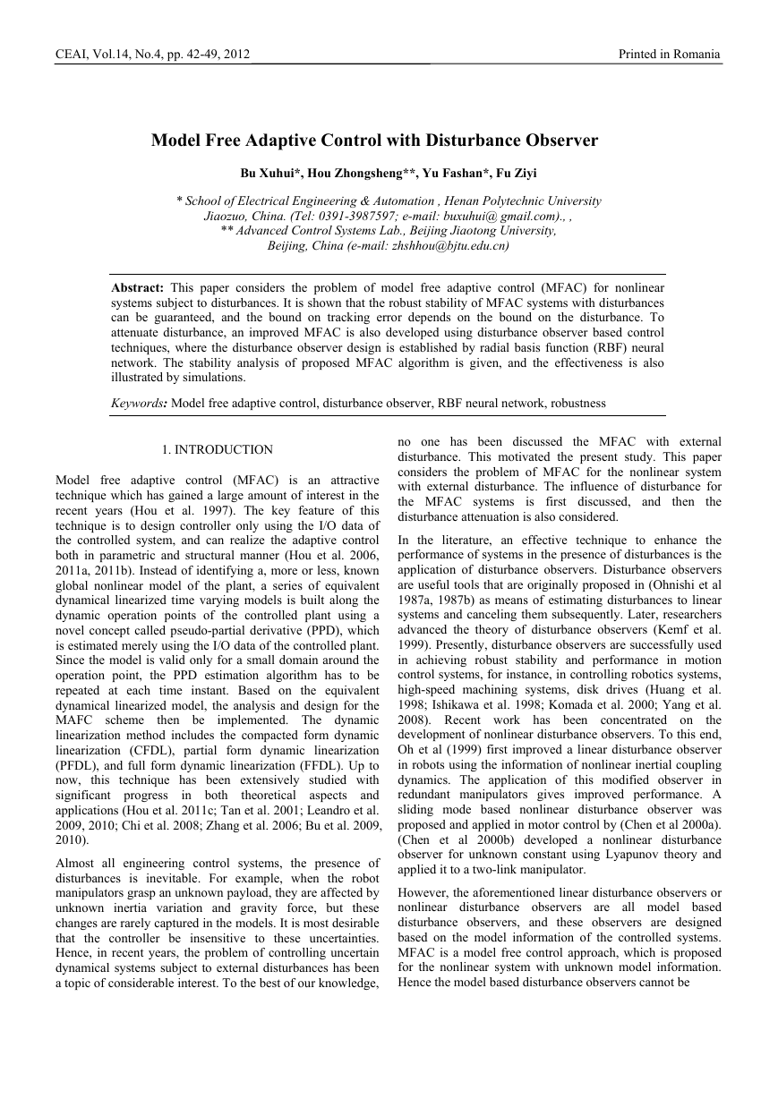(18) Theorem 2 gives Fig. 1. The configuration of MFAC with disturbances observer. 4. MFAC WITH DISTURBANCE OBSERVERS 4.1 The improved MFAC algorithm In this section, a robust MFAC for disturbance attenuation is proposed. The design procedure for disturbance attenuation is given in the following procedure: 1) Design a disturbance observer to estimate the disturbance. 2) Integrate the disturbance observer with the controller by replacing the disturbance in the MFAC algorithm with its estimation yielded by the disturbance observer. From Theorem 3, the nonlinear system (8) with disturbance can be described as y k u k ( ) (  (23) 1)   d k ( ).   k ( )  

46 CONTROL ENGINEERING AND APPLIED INFORMATICS Substituting control algorithm (7) into (23) gives y k ( 1)   y k ( )   k ( ) ˆ( ) k  ˆ( ) k     2 * y  y k ( )    d k ( ). (24) d k in the right of the Eq.(24), which Note that the term ( ) d k . As shown in Fig.1, if the results from the disturbance ( ) disturbance can be estimated, the control low with the disturbance estimated value can be designed to compensate the influence of the disturbances. Therefore, the following improved control algorithm can be given: u k ( )   y k ( * 1)   y k ( )   ˆ d k ( )  ˆ k ( )  , (25) where is the estimated valued of d k ( ) . Theorem 4: For the nonlinear system (8) with Assumptions Al, A2, A3, and using the MFAC algorithms (5), (6), (25), , are chosen as when const y k ( ) * if ,   y * 0,  (0,1) , and , satisfy  2 ) , then the b ( 4 system tracking error is bounded convergence, and the . bounded depended on the error between ˆ( ) d k d k ( ) and Proof: Substitute the control algorithm (25) into (23), that is y k ( 1)   d k ( ) y k ( ) k ( )   u k ( 1)   ˆ( ) k  ˆ k ( )    ˆ( ) d k 2   u k ( )   ˆ( ) k    ˆ k ( )      y k ( )   k ( )  d k ( )  2 * y  y k ( )   ˆ d k ( )  ˆ k ( )       (26)  y k ( )   k ( )  * y  y k ( )   k ( )  ˆ( ) k  ˆ d k ( )    d k ( ), subtracting *y in both sides of (26) gives e k (  1) 1    k ( ) k ( ), ˆ   k Since ( ), positive constant  e k ( ) k ( )  ˆ( ) k  ˆ( ), d k d k ( )   1 satisfying ˆ d k ( )    d k ( ) . (27) are bounded, it exists a small (28)     ,  1 d k ( ) ˆ( ) d k k ( )  ˆ( ) k  From Lemma 2, (27) and (28), it is obvious that e k 1) (  d e k ( ) ) (1   1 e k d ( ) (1   1 e d ) (1) (1   1 d (1 )      1 1 1  d ) (1 k 1    1 1   1 1)  (1   ) ,   1 1 d 1   2 k which leads to (29) e k lim ( ) k    1 d 1 . (30) Hence, the system tracking error is bounded convergence. 1 , which is The bounded on tracking error depends on d k determined by the error between ( ) ˆ( ) d k and . Remark 7: It is shown that the tracking error of the system is convergence when the disturbance estimated algorithm is introduced into the MFAC algorithm. The smaller tracking error can be obtained when 1 is smaller. From (28), one knows that 1 is determined by the estimated algorithm. In the following, the disturbance observer by RBF neural network is given. 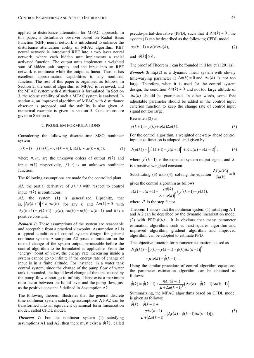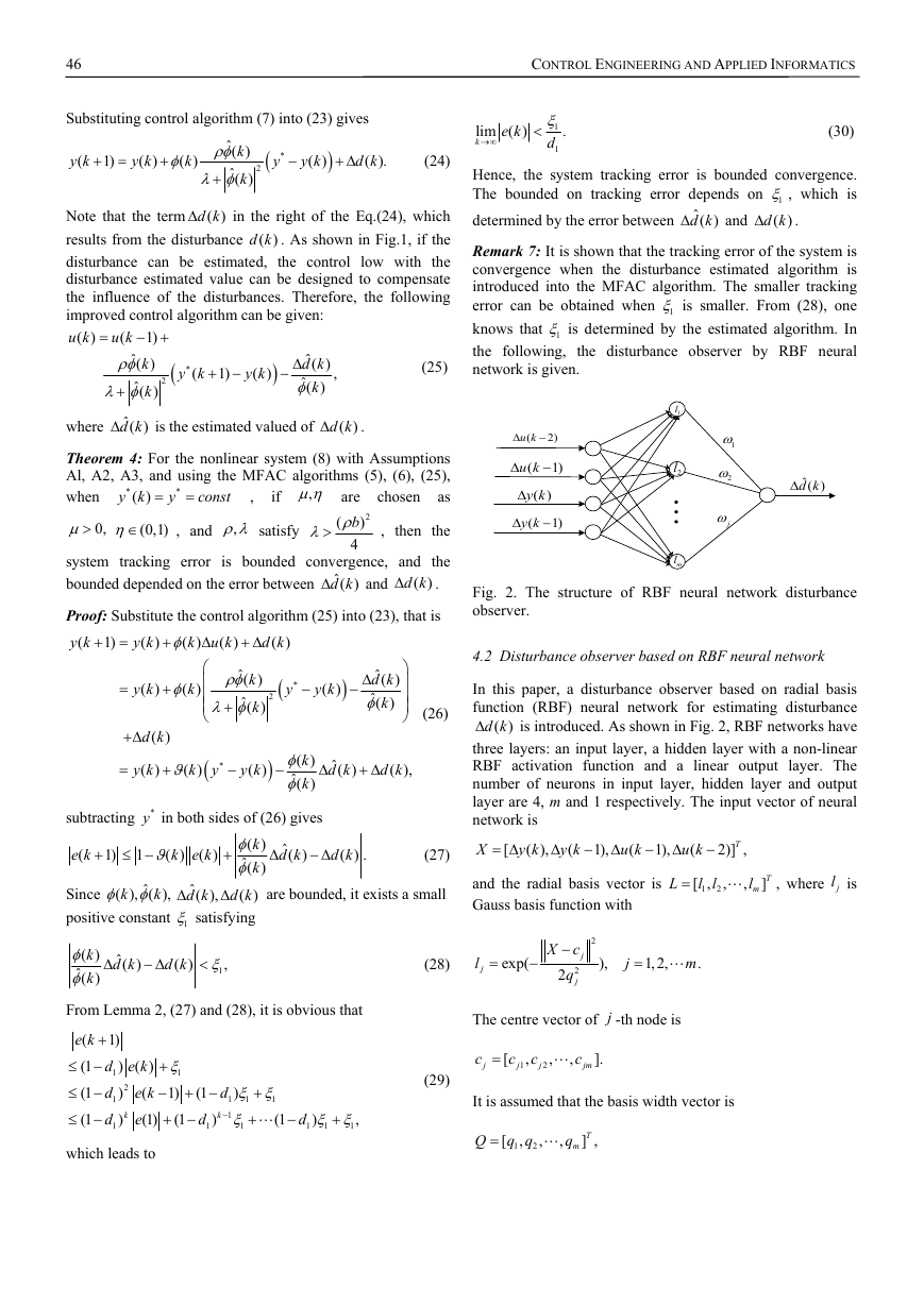u k (  2) u k (  1) y k ( ) y k (  1) 1l 2l  ml 1 2 j ˆ( )d k Fig. 2. The structure of RBF neural network disturbance observer. 4.2 Disturbance observer based on RBF neural network In this paper, a disturbance observer based on radial basis function (RBF) neural network for estimating disturbance d k is introduced. As shown in Fig. 2, RBF networks have ( ) three layers: an input layer, a hidden layer with a non-linear RBF activation function and a linear output layer. The number of neurons in input layer, hidden layer and output layer are 4, m and 1 respectively. The input vector of neural network is X y k ( ), 1),   1),   y k (  2)] ,T [   u k ( u k (  and the radial basis vector is Gauss basis function with L  l [ , 1 l 2 ,  , l m ]T , where jl is l j  exp(  2 ), j X c  q 2 2 j j   m 1,2, . The centre vector of j -th node is c j  [ c , c j 1 j 2 ,  , c jm ]. It is assumed that the basis width vector is Q q q , 2  [ 1 ,  , q m ] ,T

CONTROL ENGINEERING AND APPLIED INFORMATICS where jb is the basis width parameter of j -th node. The weight vector of network is given as W    m   [ , , , 1 2 ] ,T then, the output of the RBF neural network is ˆ( ) d k   l   2 2 l 1 1     l m m . Considering the following index J  1  2 k (  d k ( )   ˆ d k ( )) , 2 using the gradient descent approach, the following update algorithms can be obtained: j j 1 k ( ) q [     (   j  [             c [    c k ( ) ji q k ( ) j   j q k ( j k     j d k ( ) 1) [       1 k k 2)] ( 1) (     j ˆ d k l ( )] j d k ( )   ˆ d k ( )] l  j q 1)     [   1 x 1 j ˆ d k ( )]  j d k ( )   2 j j X c  q 3 j q k ( j c  q 2 j c k [ (  ji 1 ji j c k ( ji 1)      1 c ji 1)   c k ( ji  2)] , (31) q k ( j  2)] 1)   1 is learning rate, and 1 is momentum factor. It is where worth pointing out that the training of RBF network needs some sampling data. 5. SIMULATIONS In this example, the following SISO nonlinear system is considered y k (  y k 1) ( 1   y k ( u k 2) ( 1) 2   1)  y k (  y k (   2) 1    2) 2 u k ( )  d k ( ), (32) 1)  y k y k ( ) (  d k is the external disturbance and it is unknown. ( ) where The desired output is y k ( round k ( * 1)    ( 0.5) /200) ,0   k 1000. 0 Firstly, it is assumed that there is no disturbances (i.e. d k  ) and the MFAC algorithms (5)-(7) is used to ( ) control the nonlinear system (32). The initial conditions are given as the resetting initial value of PPD is 0.5, and the controller . 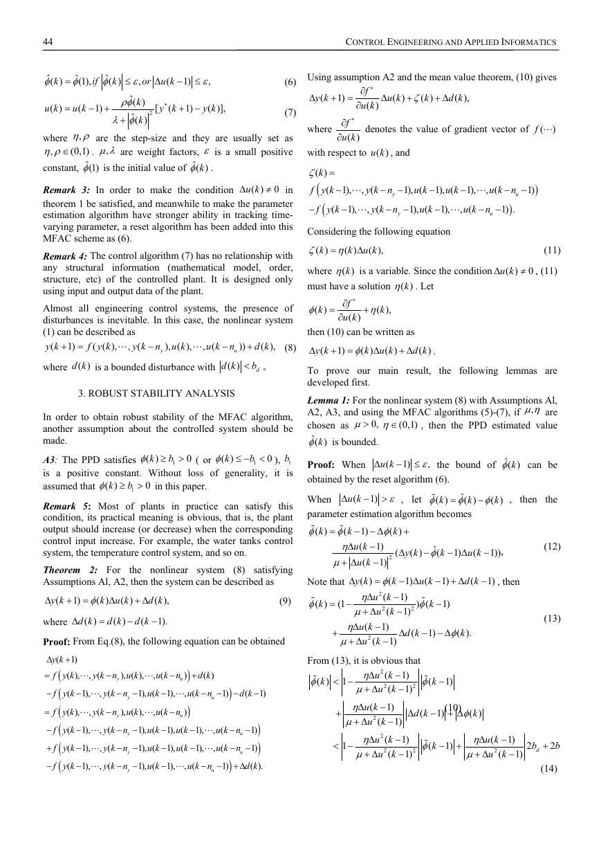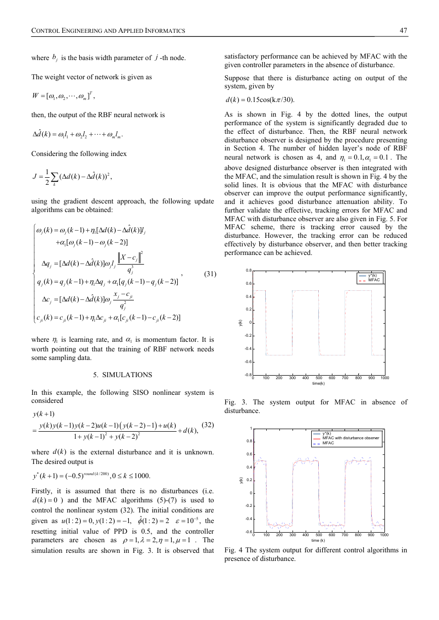The parameters are chosen as simulation results are shown in Fig. 3. It is observed that        ˆ(1: 2) (1: 2) (1: 2) 510 ,   2   0, 2, 1, 1, 1,   u    1 y 47 satisfactory performance can be achieved by MFAC with the given controller parameters in the absence of disturbance. Suppose that there is disturbance acting on output of the system, given by d k ( ) 0.15cos(k /30). 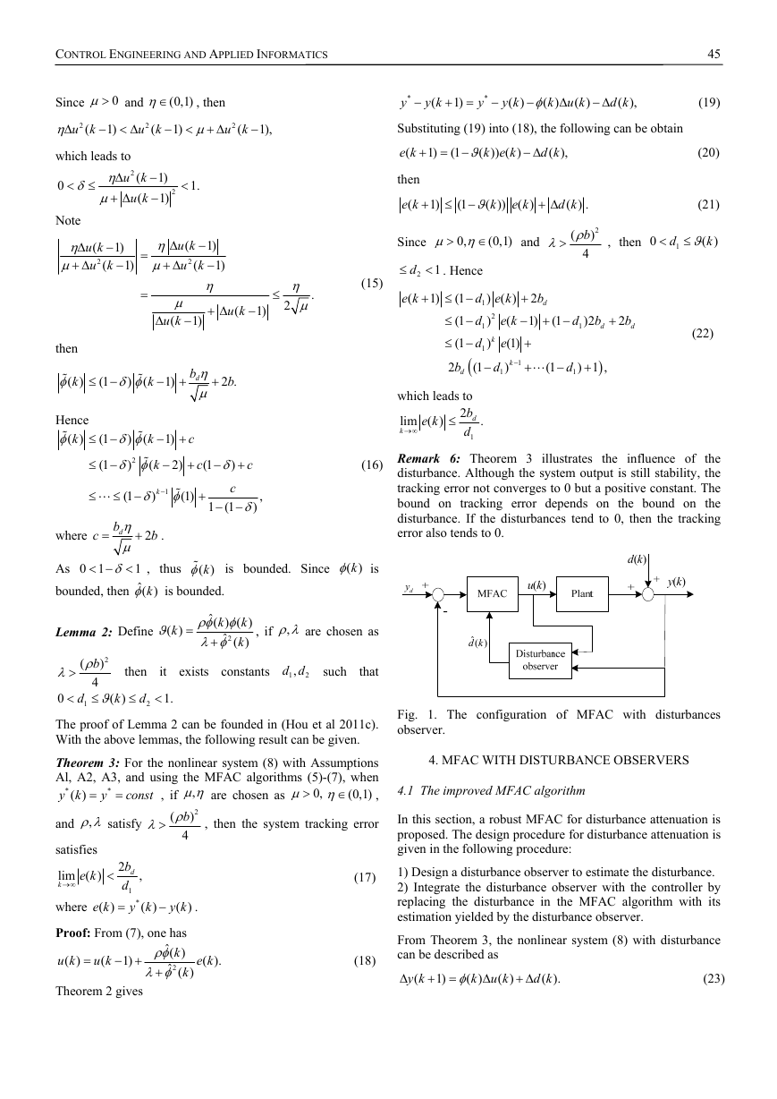    1 0.1 0.1,  1 As is shown in Fig. 4 by the dotted lines, the output performance of the system is significantly degraded due to the effect of disturbance. Then, the RBF neural network disturbance observer is designed by the procedure presenting in Section 4. The number of hidden layer’s node of RBF neural network is chosen as 4, and . The above designed disturbance observer is then integrated with the MFAC, and the simulation result is shown in Fig. 4 by the solid lines. It is obvious that the MFAC with disturbance observer can improve the output performance significantly, and it achieves good disturbance attenuation ability. 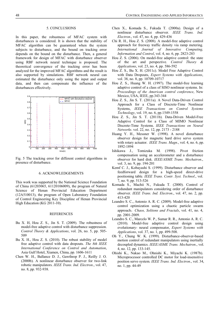To further validate the effective, tracking errors for MFAC and MFAC with disturbance observer are also given in Fig. 5. For MFAC scheme, there is tracking error caused by the disturbance. However, the tracking error can be reduced effectively by disturbance observer, and then better tracking performance can be achieved. 0.8 0.6 0.4 0.2 ) k ( y 0 -0.2 -0.4 -0.6 -0.8 0 y*(k) MFAC 100 200 300 400 500 time(k) 600 700 800 900 1000 Fig. 3. The system output for MFAC in absence of disturbance. 1 0.8 0.6 0.4 ) k ( y 0.2 0 -0.2 -0.4 -0.6 0 y*(k) MFAC with disturbance observer MFAC 100 200 300 400 500 600 700 800 900 1000 time (k) Fig. 4 The system output for different control algorithms in presence of disturbance.

CONTROL ENGINEERING AND APPLIED INFORMATICS 48 5. CONCLUSIONS In this paper, the robustness of MFAC system with disturbances is considered. It is shown that the stability of MFAC algorithm can be guaranteed when the system subjects to disturbance, and the bound on tracking error depends on the bound on the disturbance. Then, a general framework for design of MFAC with disturbance observer using RBF network neural technique is proposed. The theoretical convergence of the tracking error has been analyzed for the improved MFAC algorithms and the result is also supported by simulations. RBF network neural can estimated the disturbance only using the input and output data, and the disturbances effectively. then can compensate influence of the MFAC with disturbance observer MFAC 0.9 0.8 0.7 0.6 0.5 0.4 0.3 0.2 0.1 | ) k ( e | 0 0 100 200 300 400 500 time(k) 600 700 800 900 1000 Fig. 5 The tracking error for different control algorithms in presence of disturbance. 6. ACKNOWLEDGEMENTS This work was supported by the National Science Foundation of China (61203065, 61120106009), the program of Natural Science of Henan Provincial Education Department (12A510013), the program of Open Laboratory Foundation of Control Engineering Key Discipline of Henan Provincial High Education (KG 2011-10). REFERENCES Bu X. H, Hou Z. S., Jin S. T. (2009). The robustness of model-free adaptive control with disturbance suppression. Control Theory & Applications, vol. 26, no. 5, pp. 505- 509 Bu X. H., Hou Z. S. (2010). The robust stability of model free adaptive control with data dropouts. The 8th IEEE International Conference on Control and Automation, Asia Gulf Hotel, Xiamen, China, pp. 1606-1611 Chen W. H., Ballance D. J., Gawthrop P. J., Reilly J. O. (2000b). A nonlinear disturbance observer for two-link robotic manipulators. IEEE Trans. Ind. Electron., vol. 47, no. 8, pp. 932-938. of Chen X., Komada S., Fukuda T. (2000a). Design of a Ind. nonlinear disturbance observer. Electron., vol. 47, no. 4, pp. 429-436 IEEE Trans. Chi R. H., Hou Z. S. (2008). A model-free adaptive control approach for freeway traffic density via ramp metering. International Innovative Computing, Information and Control, vol. 4, no. 6, pp. 2823-283 Journal Hou Z. S. (2006). On model-free adaptive control: the state the art and perspective. Control Theory & of Applications, vol. 23, no. 4, pp. 586-592 Hou Z. S., Bu X. H. (2011c). Model Free Adaptive Control with Data Dropouts, Expert Systems with Applications, vol. 38, no. 8, pp. 10709-10717 Hou Z. S., Huang W. H. (1997). The model-free learning adaptive control of a class of SISO nonlinear systems. In: Proceedings of the American control conference, New Mexico, USA, IEEE, pp.343-344 Hou Z. S., Jin S. T. (2011a). A Novel Data-Driven Control Approach for a Class of Discrete-Time Nonlinear IEEE Transactions on Control Systems Systems, Technology, vol. 19, no. 6, pp.1549-1558 Hou Z. S., Jin S. T. (2011b). Data-Driven Model-Free Adaptive Control for a Class of MIMO Nonlinear Discrete-Time Systems. IEEE Transactions on Neural Networks. vol. 22, no. 12, pp. 2173 - 2188 Huang Y. H., Messner W. (1998). A novel disturbance observer design for magnetic hard drive servo system with rotary actuator. IEEE Trans. Magn., vol. 4, no. 6, pp. 1892-1894 Ishikawa J., Tomizuka M. friction compensation using an accelerometer and a disturbance observer for hard disk. IEEE/ASME Trans. Mechatron., vol. 3, no. 9, pp. 194-201 (1998). Pivot Kemf C. J., Kobayashi S. (1999). Disturbance observer and feedforward design for a high-speed direct-drive positioning table. IEEE Trans. Contr. Syst. Technol., vol. 7, no. 9, pp. 513-526 Komada S., Machii N., Fukuda T. (2000). Control of redundant manipulators considering order of disturbance observer. IEEE Trans. Ind. Electron., vol. 47, no. 2, pp. 413-420 Leandro S. C., Antonio A. R. C. (2009). Model-free adaptive control optimization using a chaotic particle swarm approach，Chaos, Solitons and Fractals, vol. 41, no. 4, pp. 2001-2009. Leandro S. C., Marcelo W. P., Sumar R. R., Antonio A. R. C. (2010). Model-free adaptive control design using evolutionary- neural compensator, Expert Systems with Applications, vol. 37, no. 1, pp. 499-508. Oh Y., Chung W. K. (1999). Disturbance-observer-based motion control of redundant manipulators using inertially decoupled dynamics. IEEE/ASME Trans. Mechatron., vol. 4, no. 12, pp. 133-145. Ohishi K., Nakao M., Ohnishi K., Miyachi K. (1987b). Microprocessor controlled DC motor for load-insensitive position servo system. IEEE Trans. Ind. Electron., vol. 34, no. 1, pp. 44-49

CONTROL ENGINEERING AND APPLIED INFORMATICS 49 Ohnishi K. (1987a). A new servo method in mechatronics. Trans. Jpn. Soc. Elect. Eng., vol. 107, no. D, pp. 83-86 Tan K. K., Lee T. H., Huang S. N., et al. (2001). Adaptive- Predictive control of a class of SISO nonlinear systems. Dynamics and Control, vol. 11, no. 2, pp. 151-174 Yang Z. J., Tsubakihara H., Kanae S., Wada K., Su C. Y. (2008). A novel robust nonlinear motion controller with disturbance observer. IEEE Trans. Control Syst. Technol. vol. 16, no. 1, pp. 137–147 Zhang B., Zhang W. D. (2006). Adaptive predictive functional control of a class of nonlinear systems, ISA Trans., vol. 45, no. 2, pp. 175-83

资料库

Model Free Adaptive Control with Disturbance Observer.pdf

相关推荐

开发技术

热门标签

最新资料