Volume �� ��� � �, pp. ��� � ���
Markov Random Fields and Images
Patrick P
erez
Irisa�Inria, Campus de Beaulieu,
����� Rennes Cedex, France
perez@irisa.fr
e-mail:
At the intersection of statistical physics and probability theory, Markov random
�elds and Gibbs distributions have emerged in the early eighties as powerful tools
for modeling images and coping with high-dimensional inverse problems from low-
level vision. Since then, they have been used in many studies from the image
processing and computer vision community. A brief and simple introduction to
the basics of the domain is proposed.
�. Introduction and general framework
With a seminal paper by Geman and Geman in � �� ����, powerful tools
known for long by physicists ��� and statisticians ��� were brought in a com-
prehensive and stimulating way to the knowledge of the image processing and
computer vision community. Since then, their theoretical richness, their prac-
tical versatility, and a number of fruitful connections with other domains, have
resulted in a profusion of studies. These studies deal either with the mod-
eling of images �for synthesis, recognition or compression purposes� or with
the resolution of various high-dimensional inverse problems from early vision
�e.g., restoration, deblurring, classi�cation, segmentation, data fusion, surface
reconstruction, optical �ow estimation, stereo matching, etc. See collections of
examples in ���, ��, ����.
The implicit assumption behind probabilistic approaches to image analysis
is that, for a given problem, there exists a probability distribution that can
capture to some extent the variability and the interactions of the di�erent sets
of relevant image attributes. Consequently, one considers the variables of the
problem as random variables forming a set �or random vector� X = �Xi�n
with joint probability distribution PX
i=�
�.
� PX is actually a probability mass in the case of discrete variables, and a probability density
function when the Xi’s are continuously valued. In the latter case, all summations over
states or con�gurations should be replaced by integrals.
���
�
The �rst critical step toward probabilistic modeling thus obviously relies on
the choice of the multivariate distribution PX . Since there is so far no really
generic theory for selecting a model, a tailor-made parameterized function P�
X
is generally chosen among standard ones, based on intuition of the desirable
properties �.
The basic characteristic of chosen distributions is their decomposition as a
product of factors depending on just a few variables �one or two in most cases�.
Also, a given distribution involves only a few types of factors.
One has simply to specify these local �interaction" factors �which might
be complex, and might involve variables of di�erent nature� to de�ne, up to
some multiplicative constant, the joint distribution PX �x�; : : : ; xn�: one ends
up with a global model.
With such a setup, each variable only directly depends on a few other �neigh-
boring" variables. From a more global point of view, all variables are mutually
dependent, but only through the combination of successive local interactions.
This key notion can be formalized considering the graph for which i and j are
neighbors if xi and xj appear within a same local component of the chosen
factorization. This graph turns out to be a powerful tool to account for local
and global structural properties of the model, and to predict changes in these
properties through various manipulations. From a probabilistic point of view,
this graph neatly captures Markov-type conditional independencies among the
random variables attached to its vertices.
After the speci�cation of the model, one deals with its actual use for mod-
eling a class of problems and for solving them. At that point, as we shall see,
one of the two following things will have to be done: ��� drawing samples from
the joint distribution, or from some conditional distribution deduced from the
joint law when part of the variables are observed and thus �xed; ��� maximiz-
ing some distribution �PX itself, or some conditional or marginal distribution
deduced from it�.
The very high dimensionality of image problems under concern usually ex-
cludes any direct method for performing both tasks. However the local decom-
position of PX fortunately allows to devise suitable deterministic or stochastic
iterative algorithms, based on a common principle: at each step, just a few
variables �often a single one� are considered, all the others being �frozen".
Markovian properties then imply that the computations to be done remain
local, that is, they only involve neighboring variables.
This paper is intended to give a brief �and de�nitely incomplete� overview
of how Markovian models can be de�ned and manipulated in the prospect of
modeling and analyzing images. Starting from the formalization of Markov ran-
dom �elds �mrfs� on graphs through the speci�cation of a Gibbs distribution
�x��, the standard issues of interest are then grossly reviewed: sampling from
a high-dimensional Gibbs distribution �x��; learning models �at least param-
eters� from observed images �x��; using the Bayesian machinery to cope with
� Superscript � denotes a parameter vector. Unless necessary, it will be dropped for nota-
tional convenience.
���
�
inverse problems, based on learned models �x��; estimating parameters with
partial observations, especially in the case of inverse problems �x��. Finally
two modeling issues �namely the introduction of so-called auxiliary variables,
and the de�nition of hierarchical models�, which are receiving a great deal of
attention from the community at the moment, are evoked �x��.
�. Gibbs distribution and graphical Markov properties
Let us now make more formal acquaintance with Gibbs distributions and their
Markov properties. Let Xi; i = �; : : : ; n, be random variables taking values
in some discrete or continuous state space �, and form the random vector
X = �X�; : : : ; Xn�T with con�guration set � = �n. All sorts of state spaces
are used in practice. More common examples are: � = f�; : : : ; ���g for �-bit
quantized luminances; � = f�; : : : ; Mg for semantic �labelings" involving M
classes; � = R for continuously-valued variables like luminance, depth, etc.;
� = f�umax; : : : ; umaxg � f�vmax; : : : ; vmaxg in matching problems involving
displacement vectors or stereo disparities for instance; � = R� in vector �eld-
based problems like optical �ow estimation or shape-from-shading.
As said in the introduction, PX exhibits a factorized form:
PX �x� � Yc�C
fc�xc�;
���
where C consists of small index subsets c, the factor fc depends only on the
variable subset xc = fxi; i � cg, and Qc fc is summable over �. If, in addi-
tion, the product is positive ��x � �; PX �x� � ��, then it can be written in
exponential form �letting Vc = � ln fc�:
PX �x� =
�
Z
expf�Xc
Vc�xc�g:
���
Well known from physicists, this is the Gibbs �or Boltzman� distribution with
interaction potential fVc; c � Cg, energy U =Pc Vc, and partition function �of
parameters� Z = Px�� expf�U �x�g
the more likely, whereas high energies correspond to low probabilities.
�. Con�gurations of lower energies are
The interaction structure induced by the factorized form is conveniently
captured by a graph that statisticians refer to as the independence graph: the
independence graph associated with the factorization Qc�C fc is the simple
undirected graph G = �S; E� with vertex set S = f�; : : : ; ng, and edge set E
de�ned as: fi; jg � E �� c � C : fi; jg � c, i.e., i and j are neighbors if xi
and xj appear simultaneously within a same factor fc. The neighborhood n�i�
�. As a consequence
of site i is then de�ned as n�i� = fj � S : fi; jg � Eg
� Formal expression of the normalizing constant Z must not veil the fact that it is unknown
and beyond reach in general, due to the intractable summation over �.
� n = fn�i�; i � Sg is called a neighborhood system, and the neighborhood of some subset
a � S is de�ned as n�a� = fj � S � a : n�j� � a �= �g.
���
�
of the de�nition, any subset c is either a singleton or composed of mutually
neighboring sites: C is a set of cliques for G .
When variables are attached to the pixels of an image, the most common
neighborhood systems are the regular ones where a site away from the border
of the lattice has four or eight neighbors. In the �rst case ��rst-order neighbor-
hood system, like in Figure �.a� subsets c have at most two elements, whereas,
in the second-order neighborhood system cliques can exhibit up to � sites. How-
ever, other graph structures are also used: in segmentation applications where
the image plane is partitioned, G might be the planar graph associated to the
partition �Figure �.b�; and hierarchical image models often live on �quad�-trees
�Figure �.c�.
(a)
(b)
(c)
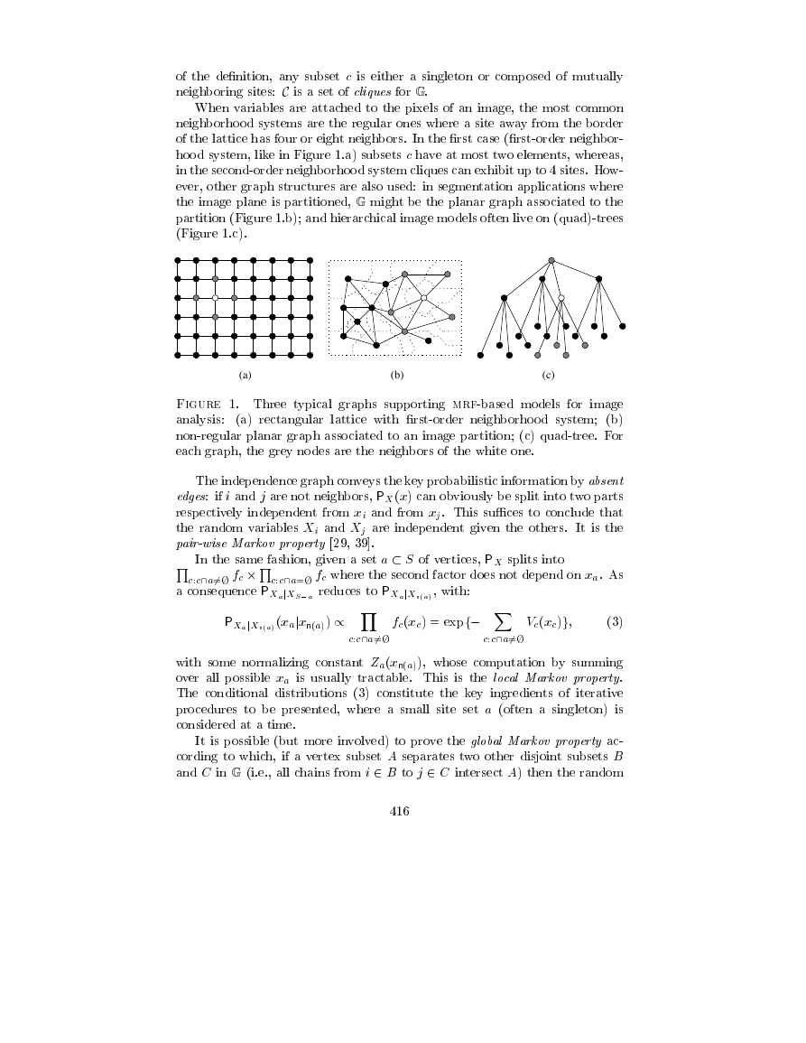
Figure �. Three typical graphs supporting mrf-based models for image
analysis:
�a� rectangular lattice with �rst-order neighborhood system; �b�
non-regular planar graph associated to an image partition; �c� quad-tree. For
each graph, the grey nodes are the neighbors of the white one.
The independence graph conveys the key probabilistic information by absent
edges: if i and j are not neighbors, PX �x� can obviously be split into two parts
respectively independent from xi and from xj. This su�ces to conclude that
the random variables Xi and Xj are independent given the others. It is the
pair-wise Markov property �� , � �.
In the same fashion, given a set a � S of vertices, PX splits into
Qc:c�a�=� fc �Qc:c�a=� fc where the second factor does not depend on xa. As
a consequence PXajXS�a reduces to PXajXn�a� , with:
PXajXn�a� �xajxn�a�� � Yc:c�a�=�
fc�xc� = expf� Xc:c�a�=�
Vc�xc�g;
���
with some normalizing constant Za�xn�a��, whose computation by summing
over all possible xa is usually tractable. This is the local Markov property.
The conditional distributions ��� constitute the key ingredients of iterative
procedures to be presented, where a small site set a �often a singleton� is
considered at a time.
It is possible �but more involved� to prove the global Markov property ac-
cording to which, if a vertex subset A separates two other disjoint subsets B
and C in G �i.e., all chains from i � B to j � C intersect A� then the random
���
�
vectors XB and XC are independent given XA �� , � �. It can also be shown
that the three Markov properties are equivalent for strictly positive distribu-
tions. Conversely, if a positive distribution PX ful�lls one of these Markov
properties w.r.t. graph G �X is then said to be a mrf on G �, then PX is a
Gibbs distribution of the form ��� relative to the same graph. This equivalence
constitutes the Hammersley-Cli�ord theorem ���.
To conclude this section, we introduce two very standard Markov random
�elds which have been extensively used for image analysis purposes.
Example �: Ising mrf.
Introduced in the twenties in statistical physics of
condensed matter, and studied since then with great attention, this model
Its simpler
deals with binary variables �� = f��; �g� that interact locally.
formulation is given by energy
U �x� = ��Xhi;ji
xixj ;
where summation is taken over all edges hi; ji � E of the chosen graph. The
�attractive" version �� � �� statistically favors identity of neighbors. The
conditional distribution at site i is readily deduced:
PXi jXn�i� �xijxn�i�� =
expf�xiPj�n�i� xjg
� cosh��Pj�n�i� xj�
:
The Ising model is useful in detection-type problems where binary variables
are to be recovered. Some other problems �essentially segmentation and clas-
si�cation� require the use of symbolic �discrete� variables with more than two
possible states. For these cases, the Potts model also stemming from statistical
physics ���, provides an immediate extension of the Ising model, with energy
�
U �x� = ��Phi;ji����xi; xj � � ��, where � is the Kronecker delta.
Example �: Gauss-Markov �eld. It is a continuously-valued random vector
�� = R� ruled by a multivariate Gaussian distribution
PX �x� =
expf�
�
�
�x � ��T ����x � ��g;
�
pdet�����
with expectation vector E�X� = � and covariance matrix �. The �Markovian-
ity" shows up when each variable only interacts with a few others through the
quadratic energy, that is, when the matrix A = ��� is sparse. Sites i and
j are then neighbors in G i� the corresponding entry aij = aji is non-null.
Graph G is exactly the so-called structure of sparse matrix A ����. In practice
a Gauss-Markov �eld is often de�ned simply by its quadratic energy function
U �x� = �
� xi � bi�xi, with b � Rn and
A a sparse symmetric de�nite positive matrix. In that case, the expectation
which corresponds to the most probable con�guration, is the solution of the
large sparse linear system A� = b.
� xT Ax � xT b = Phi;ji aij xixj +Pi� aii
���
�
Note that in the Gaussian case, any conditional or marginal distribution
taken from PX is Gaussian and can be explicitly written down by using ad-
equate block partitioning of A and b �� , ��, � �. All Markovian properties
can then be directly deduced from this. Site-wise conditional distributions in
particular turn out to be Gaussian laws
�XijXn�i� = xn�i�� � N �
�
aii
�bi � Xj�n�i�
aij xj �; a��
ii � :
At this point, it is worth emphasizing the di�erence with so-called simultaneous
autoregressive models ��� de�ned by:
�i aiiXi = bi � Xj�n�i�
aij Xj + Wi ;
with Wi’s being i.i.d. reduced zero-mean Gaussian variables. As a fact, the
resulting inverse covariance matrix of X in this case is AT A, whose �lling
structure is larger than the one of A.
The nice properties of Gaussian mrfs, inherited from the quadratic form
of their energy, make them the more popular models in case of continuous or
�almost continuous" �i.e., j�j very large� variables.
�
�. Sampling from Gibbs distributions
In order to visually evaluate the statistical properties of the speci�ed model,
or simply to get synthetic images, one might want to draw the samples from
the distribution PX . A more important and technical reason for which this
sampling can be of much help is that for all issues requiring an exhaustive
visit of con�guration set � �intractable in practice�, e.g., summation or maxi-
mization over all possible occurrences, an approximate way to proceed consists
in randomly visiting � for long enough according to distribution PX . These
approximation methods belong to the class of Monte Carlo methods ���, ���.
The dimensionality of the model makes sampling delicate �starting with
the fact that normalizing constant Z is beyond reach�. One has to resort to a
Markov chain procedure on � which allows to sample successively from random
�elds whose distributions get closer and closer to the target distribution PX .
The locality of the model indeed permits to design a chain of random vectors
X �; : : : ; X m; : : : , without knowing Z, and such that PXm tends to PX �for
some distance� as m goes to in�nity, whatever initial distribution PX � is. The
crux of the method lies in the design of transition probabilities PXm+�jXm based
only on local conditional distributions stemming from PX , and such that the
resulting Markov chain is irreducible �, aperiodic �, and preserves the target
� There is a non-null probability to get from any x to any x� within a �nite number of
transitions: m : P
Xm
jX � �x�jx� � �.
� Con�guration set cannot be split in subsets that would be visited in a periodic way:
@ d � � : � = �d��
k=��k with X � � �� � Xm � �m�dbm=dc; �m
���
�
distribution, i.e., Px��� PXm+�jXm�xjx��PX �x�� = PX �x� for any con�guration
x � �. The latter condition is especially met when the so-called �detailed
balance" holds: PXm+�jXm�xjx��PX �x�� = PXm+�jXm�x�
Various suitable dynamics can be designed ����. A quite popular one for
image models is the Gibbs sampler ���� which directly uses conditional distribu-
tions from PX to generate the transitions. More precisely S is split into small
pieces �often singletons�, which are �visited" either at random, or according
to some pre-de�ned schedule. If a is the concerned set of sites at step m, and
x the realization of X m, a realization of X m+� is obtained by replacing xa in
x = �xa; xS�a� by x�
a, according to the conditional law
jx�PX �x�.
PXa jXS�a�:jxS�a� = PXa jXn�a� �:jxn�a��
�this law of a few variables can be exactly derived, unlike PX �. The chain thus
sampled is clearly irreducible and aperiodic �the null transition x ! x is always
possible�, and detailed balance is veri�ed since
PXm+�jXm�x�
a; xS�ajxa; xS�a�PX �xa; xS�a� =
= PXa jXS�a�x�
ajxS�a�PX �xa; xS�a�
=
PX �x�
a; xS�a�PX �xa; xS�a�
PXS�a �xS�a�
is symmetric in xa and x�
a.
From a practical point of view the chain thus designed is started from any
con�guration x�, and run for a large number of steps. For m large enough, it
has almost reached an equilibrium around PX , and following con�gurations can
be considered as �non-independent� samples from PX . The decision whether
equilibrium is reached is intricate, though. The design of criteria and indicators
to answer this question is an active area of research in mcmc studies.
If the expectation of some function f of X has to be evaluated, ergodicity
. Practically, given a
properties yield E�f �X�� = limm!+�
large but �nite realization of the chain, one gets rid of the �rst m� out-of-
equilibrium samples, and computes an average over the remainder:
f �x��+:::+f �xm���
m
E �f �X�� �
�
m� � m�
m�
Xm=m�+�
f �xm� :
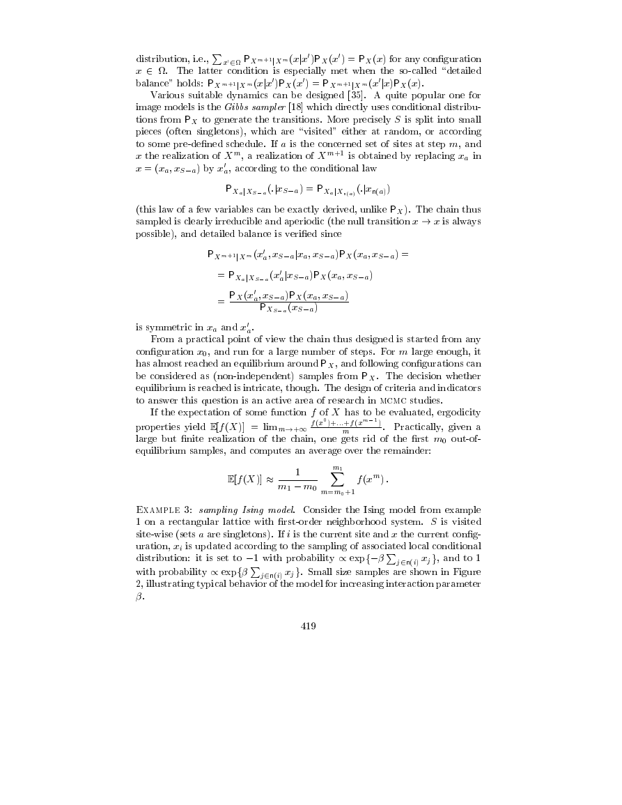
Example �: sampling Ising model. Consider the Ising model from example
� on a rectangular lattice with �rst-order neighborhood system. S is visited
site-wise �sets a are singletons�. If i is the current site and x the current con�g-
uration, xi is updated according to the sampling of associated local conditional
distribution: it is set to �� with probability � expf��Pj�n�i� xjg, and to �
with probability � expf�Pj�n�i� xjg. Small size samples are shown in Figure
�, illustrating typical behavior of the model for increasing interaction parameter
�.
��
�
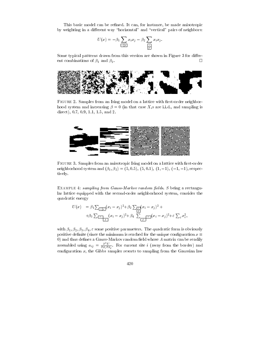
This basic model can be re�ned. It can, for instance, be made anisotropic
by weighting in a di�erent way �horizontal" and �vertical" pairs of neighbors:
U �x� = ���Xi j
xixj � ��Xi
j
xixj :
Some typical patterns drawn from this version are shown in Figure � for di�er-
ent combinations of �� and ��.
�
Figure �. Samples from an Ising model on a lattice with �rst-order neighbor-
hood system and increasing � = � �in that case Xis are i.i.d., and sampling is
direct�, �.�, �. , �.�, �.�, and �.
Figure �. Samples from an anisotropic Ising model on a lattice with �rst-order
neighborhood system and ���; ��� = ��; �:��; ��; �:��; ��; ���; ���; ���, respec-
tively.
Example �: sampling from Gauss-Markov random �elds. S being a rectangu-
lar lattice equipped with the second-order neighborhood system, consider the
quadratic energy
U �x� = ��P i j �xi � xj��+��P i
j
�xi � xj �� +
+��P i
j
�xi � xj��+�� P i
j
�xi � xj��+"Pi x�
i ;
with ��; ��; ��; ��; " some positive parameters. The quadratic form is obviously
positive de�nite �since the minimum is reached for the unique con�guration x �
�� and thus de�nes a Gauss-Markov random �eld whose A matrix can be readily
assembled using aij = @ �U
. For current site i �away from the border� and
@xi@xj
con�guration x, the Gibbs sampler resorts to sampling from the Gaussian law
���
�




 2023年江西萍乡中考道德与法治真题及答案.doc
 2012年重庆南川中考生物真题及答案.doc
 2013年江西师范大学地理学综合及文艺理论基础考研真题.doc
 2020年四川甘孜小升初语文真题及答案I卷.doc
 2020年注册岩土工程师专业基础考试真题及答案.doc
 2023-2024学年福建省厦门市九年级上学期数学月考试题及答案.doc
 2021-2022学年辽宁省沈阳市大东区九年级上学期语文期末试题及答案.doc
 2022-2023学年北京东城区初三第一学期物理期末试卷及答案.doc
 2018上半年江西教师资格初中地理学科知识与教学能力真题及答案.doc
 2012年河北国家公务员申论考试真题及答案-省级.doc
 2020-2021学年江苏省扬州市江都区邵樊片九年级上学期数学第一次质量检测试题及答案.doc
 2022下半年黑龙江教师资格证中学综合素质真题及答案.doc