Topics in Multi-User Information Theory.pdf-资料库

JIAJIA0386-2576451-Topics in Multi-User Information Theory.pdf-第1页.png

第1页 / 共180页

JIAJIA0386-2576451-Topics in Multi-User Information Theory.pdf-第2页.png

第2页 / 共180页

JIAJIA0386-2576451-Topics in Multi-User Information Theory.pdf-第3页.png

第3页 / 共180页

JIAJIA0386-2576451-Topics in Multi-User Information Theory.pdf-第4页.png

第4页 / 共180页

JIAJIA0386-2576451-Topics in Multi-User Information Theory.pdf-第5页.png

第5页 / 共180页

JIAJIA0386-2576451-Topics in Multi-User Information Theory.pdf-第6页.png

第6页 / 共180页

JIAJIA0386-2576451-Topics in Multi-User Information Theory.pdf-第7页.png

第7页 / 共180页

JIAJIA0386-2576451-Topics in Multi-User Information Theory.pdf-第8页.png

第8页 / 共180页

Foundations and Trends R! in Communications and Information Theory Vol. 4, Nos. 4–5 (2007) 265–444 c! 2008 G. Kramer DOI: 10.1561/0100000028 Topics in Multi-User Information Theory Gerhard Kramer Bell Laboratories, Alcatel-Lucent, 600 Mountain Avenue, Murray Hill, New Jersey, 07974, USA, gkr@bell-labs.com Abstract This survey reviews fundamental concepts of multi-user information theory. Starting with typical sequences, the survey builds up knowl- edge on random coding, binning, superposition coding, and capacity converses by introducing progressively more sophisticated tools for a selection of source and channel models. The problems addressed include: Source Coding; Rate-Distortion and Multiple Descriptions; Capacity-Cost; The Slepian–Wolf Problem; The Wyner-Ziv Problem; The Gelfand-Pinsker Problem; The Broadcast Channel; The Multiac- cess Channel; The Relay Channel; The Multiple Relay Channel; and The Multiaccess Channel with Generalized Feedback. The survey also includes a review of basic probability and information theory.

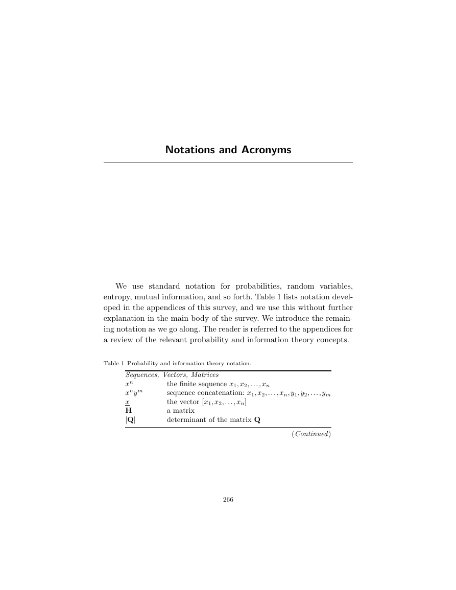
Notations and Acronyms We use standard notation for probabilities, random variables, entropy, mutual information, and so forth. Table 1 lists notation devel- oped in the appendices of this survey, and we use this without further explanation in the main body of the survey. We introduce the remain- ing notation as we go along. The reader is referred to the appendices for a review of the relevant probability and information theory concepts. Table 1 Probability and information theory notation. Sequences, Vectors, Matrices xn xnym x H |Q| the ﬁnite sequence x1, x2, . . . , xn sequence concatenation: x1, x2, . . . , xn, y1, y2, . . . , ym the vector [x1, x2, . . . , xn] a matrix determinant of the matrix Q (Continued) 266

Notations and Acronyms 267 Table 1 (Continued) Probability Pr[A] Pr[A|B] PX(·) PX|Y (·) supp(PX) pX(·) pX|Y (·) E [X] E [X|A] Var[X] QX probability of the event A probability of event A conditioned on event B probability distribution of the random variable X probability distribution of X conditioned on Y support of PX probability density of the random variable X probability density of X conditioned on Y expectation of the real-valued X expectation of X conditioned on event A variance of X covariance matrix of X Information Theory H(X) H(X|Y ) I(X; Y ) I(X; Y |Z) D(PX!PY ) h(X) h(X|Y ) H2(·) entropy of the discrete random variable X entropy of X conditioned on Y mutual information between X and Y mutual information between X and Y conditioned on Z informational divergence between PX and PY diﬀerential entropy of X diﬀerential entropy of X conditioned on Y binary entropy function

1 Typical Sequences and Source Coding 1.1 Typical Sequences Shannon introduced the notion of a “typical sequence” in his 1948 paper “A Mathematical Theory of Communication” [55]. To illustrate the idea, consider a discrete memoryless source (DMS), which is a device that emits symbols from a discrete and ﬁnite alphabet X in an inde- pendent and identically distributed (i.i.d.) manner (see Figure 1.1). Suppose the source probability distribution is PX(·) where PX(0) = 2/3 and PX(1) = 1/3. (1.1) Consider the following experiment: we generated a sequence of length 18 by using a random number generator with the distribution (1.1). We write this sequence below along with three other sequences that we generated artiﬁcially. (a) 0, 0, 0, 0, 0, 0, 0, 0, 0, 0, 0, 0, 0, 0, 0, 0, 0, 0 (b) 1, 0, 1, 1, 0, 1, 0, 1, 1, 1, 0, 0, 0, 0, 1, 0, 1, 0 (c) 0, 0, 0, 1, 1, 0, 0, 1, 0, 0, 1, 1, 0, 0, 0, 1, 1, 0 (d) 1, 1, 1, 1, 1, 1, 1, 1, 1, 1, 1, 1, 1, 1, 1, 1, 1, 1. 268

1.2 Entropy-Typical Sequences 269 DMS Fig. 1.1 A discrete memoryless source with distribution PX(·). If we compute the probabilities that these sequences were emitted by the source (1.1), we have (a) (2/3)18 · (1/3)0 ≈ 6.77 · 10−4 (b) (2/3)9 · (1/3)9 ≈ 1.32 · 10−6 (c) (2/3)11 · (1/3)7 ≈ 5.29 · 10−6 (d) (2/3)0 · (1/3)18 ≈ 2.58 · 10−9. Thus, the ﬁrst sequence is the most probable one by a large margin. However, the reader will likely not be surprised to ﬁnd out that it is sequence (c) that was actually put out by the random number genera- tor. Why is this intuition correct? To explain this, we must deﬁne more precisely what one might mean by a “typical” sequence. 1.2 Entropy-Typical Sequences Let xn be a ﬁnite sequence whose ith entry xi takes on values in X . We write X n for the Cartesian product of the set X with itself n times, i.e., we have xn ∈X n. Let N(a|xn) be the number of positions of xn having the letter a, where a ∈X . There are several natural deﬁnitions for typical sequences. Shannon in [55, Sec. 7] chose a deﬁnition based on the entropy of a random variable X. Suppose that X n is a sequence put out by the DMS PX(·), which means that PXn(xn) =!n i=1 PX(xi) is the probability that xn was put out by the DMS PX(·). More generally, we will use the notation (1.2) PX(xi). X(xn) = P n n"i=1 We further have P n X(xn) =#!a∈supp(PX) PX(a)N(a|xn) 0 if N(a|xn) = 0 whenever PX(a) = 0 else (1.3)

270 Typical Sequences and Source Coding 1 n − log2 P n and intuitively one might expect that the letter a occurs about X(xn) ≈ Πa∈supp(PX)PX(a)nPX(a) or N(a|xn) ≈ nPX(a) times, so that P n X(xn) ≈ $a∈supp(PX) %%%% Shannon therefore deﬁned a sequence xn to be typical with respect to and PX(·) if − H(X)%%%% < −PX(a)log2 PX(a). for some small positive . The sequences satisfying (1.4) are sometimes called weakly typical sequences or entropy-typical sequences [19, p. 40]. We can equivalently write (1.4) as 2−n[H(X)+] < P n X(xn) < 2−n[H(X)−]. (1.5) X(xn) −log2 P n n (1.4) Example 1.1. If PX(·) is uniform then for any xn we have X(xn) = |X|−n = 2−nlog2 |X| = 2−nH(X) P n (1.6) and all sequences in X n are entropy-typical. Example 1.2. The source (1.1) has H(X) ≈ 0.9183 and the above four sequences are entropy-typical with respect to PX(·) if (a) > 1/3 (b) > 1/6 (c) > 1/18 (d) > 2/3. Note that sequence (c) requires the smallest . We remark that entropy typicality applies to continuous random X(xn) in (1.4) X(xn). In contrast, the next deﬁnition can be variables with a density if we replace the probability P n with the density value pn used only for discrete random variables.

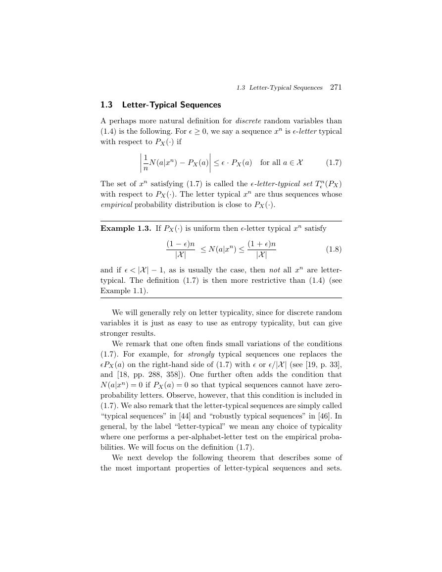
1.3 Letter-Typical Sequences 1.3 Letter-Typical Sequences 271 A perhaps more natural deﬁnition for discrete random variables than (1.4) is the following. For ≥ 0, we say a sequence xn is -letter typical with respect to PX(·) if for all a ∈X (1.7) %%%% 1 n N(a|xn) − PX(a)%%%% ≤ · PX(a) The set of xn satisfying (1.7) is called the -letter-typical set T n (PX) with respect to PX(·). The letter typical xn are thus sequences whose empirical probability distribution is close to PX(·). Example 1.3. If PX(·) is uniform then -letter typical xn satisfy (1 − )n |X| ≤ N(a|xn) ≤ (1 + )n |X| (1.8) and if < |X| − 1, as is usually the case, then not all xn are letter- typical. The deﬁnition (1.7) is then more restrictive than (1.4) (see Example 1.1). We will generally rely on letter typicality, since for discrete random variables it is just as easy to use as entropy typicality, but can give stronger results. We remark that one often ﬁnds small variations of the conditions (1.7). For example, for strongly typical sequences one replaces the PX(a) on the right-hand side of (1.7) with or /|X| (see [19, p. 33], and [18, pp. 288, 358]). One further often adds the condition that N(a|xn) = 0 if PX(a) = 0 so that typical sequences cannot have zero- probability letters. Observe, however, that this condition is included in (1.7). We also remark that the letter-typical sequences are simply called “typical sequences” in [44] and “robustly typical sequences” in [46]. In general, by the label “letter-typical” we mean any choice of typicality where one performs a per-alphabet-letter test on the empirical proba- bilities. We will focus on the deﬁnition (1.7). We next develop the following theorem that describes some of the most important properties of letter-typical sequences and sets.

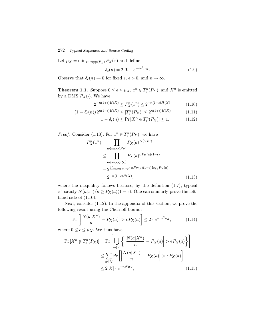
272 Typical Sequences and Source Coding Let µX = minx∈supp(PX) PX(x) and deﬁne δ(n) = 2|X| · e−n2µX . Observe that δ(n) → 0 for ﬁxed , > 0, and n → ∞. Theorem 1.1. Suppose 0 ≤ ≤ µX, xn ∈ T n by a DMS PX(·). We have 2−n(1+)H(X) ≤ P n (1 − δ(n))2n(1−)H(X) ≤| T n X(xn) ≤ 2−n(1−)H(X) (PX)|≤ 2n(1+)H(X) (PX)] ≤ 1. 1 − δ(n) ≤ Pr[X n ∈ T n (PX), and X n is emitted (1.9) (1.10) (1.11) (1.12) P n (PX), we have PX(a)N(a|xn) Proof. Consider (1.10). For xn ∈ T n X(xn) = "a∈supp(PX) ≤ "a∈supp(PX) = 2!a∈supp(PX ) nPX(a)(1−)log2 PX(a) = 2−n(1−)H(X), PX(a)nPX(a)(1−) (1.13) where the inequality follows because, by the deﬁnition (1.7), typical xn satisfy N(a|xn)/n ≥ PX(a)(1 − ). One can similarly prove the left- hand side of (1.10). Next, consider (1.12). In the appendix of this section, we prove the following result using the Chernoﬀ bound: where 0 ≤ ≤ µX. We thus have Pr[X n /∈ T n Pr&%%%% (1.14) N(a|X n) n − PX(a)%%%% > PX(a)’ ≤ 2 · e−n2µX , (PX)] = Pr()a∈X#%%%% − PX(a)%%%% > PX(a)*+ − PX(a)%%%% > PX(a)’ Pr&%%%% ≤$a∈X ≤ 2|X| · e−n2µX , n N(a|X n) N(a|X n) n (1.15)

资料库

Topics in Multi-User Information Theory.pdf

相关推荐

课程资源

热门标签

最新资料