lof
April 23, 2014
1
Improving performance of Local outlier factor with KD-Trees
Local outlier factor (LOF) is an outlier detection algorithm, that detects outliers based on comparing local
density of data instance with its neighbors. It does so to decide if data instance belongs to region of similar
density. It can detect an outlier in a dataset, for which number of clusters is unknown, and clusters are
of different density and size. It’s inspired from KNN (K-Nearest Neighbors) algorithm, and is widely used.
There is a R implemantation available.
The naive approach to do this is to form all pair euclidan distance matrix, and then run knn query to
proceed further. But this approach just sucks, as it is Θ(n2) in terms of both space and time complexity.
But, this can be improvd with KDTrees., and already its implementation exists in python, thanks to scipy,
so lets use this to find outliers.
Synthetic dataset
In [229]: %pylab inline
import numpy as np
np.random.seed(2) # to reproduce the result
Populating the interactive namespace from numpy and matplotlib
WARNING: pylab import has clobbered these variables: [’dist’]
‘%pylab --no-import-all‘ prevents importing * from pylab and numpy
In [230]: dim = 2 # number of dimensions of dataset = 2
# cluster of normal random variable moderately dense
data1 = np.random.np.random.multivariate_normal([0, 1500], [[100000, 0], [0, 100000]], 2000)
# very dense
data2 = np.random.np.random.multivariate_normal([2000, 0], [[10000, 0], [0, 10000]], 2500)
# sparse
data3 = np.random.np.random.multivariate_normal([2500, 2500], [[100000, 0], [0, 100000]], 500)
# mix the three dataset and shuffle
data = np.vstack((np.vstack((data1, data2)), data3))
np.random.shuffle(data)
# add some noise : zipf is skewed distribution and can have extreme values(outliers)
zipf_alpha = 2.25
noise = np.random.zipf(zipf_alpha, (5000,dim)) * np.sign((np.random.randint(2, size = (5000, dim)) - 0.5))
data += noise
1
�
Naive approach to LOF Pairwise Euclidean distance calculation with DistanceMetric implementation
in scikit-learn. In this, we just compute all-pair euclidean distance, i.e. d(i, j) = x(i) − x(j)2.
In [231]: from sklearn.neighbors import DistanceMetric
# distance between points
import time
tic = time.time()
dist = DistanceMetric.get_metric(’euclidean’).pairwise(data)
print ’++ took %g msecs for Distance computation’ %
((time.time() - tic)* 1000)
++ took 740 msecs for Distance computation
Performing KNN query.In this step, the nearest k neighbors are identified Nk(i), and radius is the distance
of k-th rearest neighbor of a datapoint.
In [232]: tic = time.time()
r(i) = max
k∈Nk(i)
d(i, k)
k = 17 # number of neighbors to consider
# get the radius for each point in dataset (distance to kth nearest neighbor)
# radius is the distance of kth nearest point for each point in dataset
idx_knn = np.argsort(dist, axis=1)[:,1 : k + 1] # by row’ get k nearest neighbour
radius = np.linalg.norm(data - data[idx_knn[:, -1]], axis = 1) # radius
print ’+++ took %g msecs for KNN Querying’ %
((time.time() - tic)* 1000)
+++ took 4800 msecs for KNN Querying
Then LRD(Local Reachability distance) is calculated. For this, first reach distance rd(i, j) is com-
puted between point concern x(i) and its neighbors $ j:j∈ N k(i), which is the maximum of eu-
clidean distance or radius r(i)$of pointconcerned.T hen, LRDistheinverseof meanof reachdistanceof allk −
neighborsof eachpoint.rd(i, j) = max{d(i, j), r(i)}f or j ∈ Nk(i)
|Nk(i)|
LRD(i) =
j∈Nk(i) rd(i, j)
In [233]: # calculate the local reachability density
tic = time.time()
LRD = []
for i in range(idx_knn.shape[0]):
LRD.append(np.mean(np.maximum(dist[i, idx_knn[i]], radius[idx_knn[i]])))
print ’++++ took %g msecs for LRD computation’ % ((time.time() - tic)* 1000)
++++ took 429 msecs for LRD computation
finally, the outlier score LOF is calsulated.
In [234]: # calculating the outlier score
LOF (i) =
j∈Nk(i)
LRD(j)
LRD(i)
|Nk(i)|
tic = time.time()
rho = 1. / np.array(LRD) # inverse of density
outlier_score = np.sum(rho[idx_knn], axis = 1)/ np.array(rho, dtype = np.float16)
outlier_score *= 1./k
print ’+++++ took %g msecs for Outlier scoring’ %
((time.time() - tic)* 1000)
2
�
+++++ took 9.99999 msecs for Outlier scoring
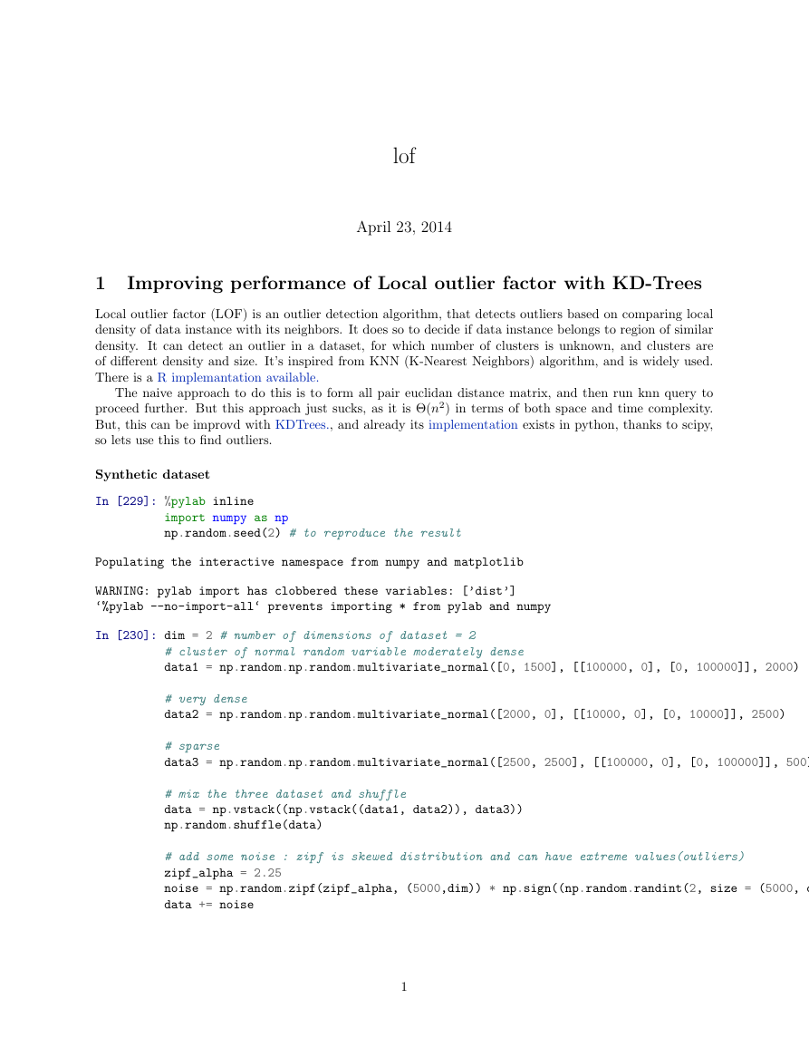
Now lets se the histogram of Outlier score, to choose the optimal threshold to decid weather a data-point
is outlier is not.
In [235]: weights = np.ones_like(outlier_score)/outlier_score.shape[0] # to normalize the histogram to probability plot
hist(outlier_score, bins = 50, weights = weights, histtype = ’stepfilled’, color = ’cyan’)
title(’Distribution of outlier score’)
Out[235]:
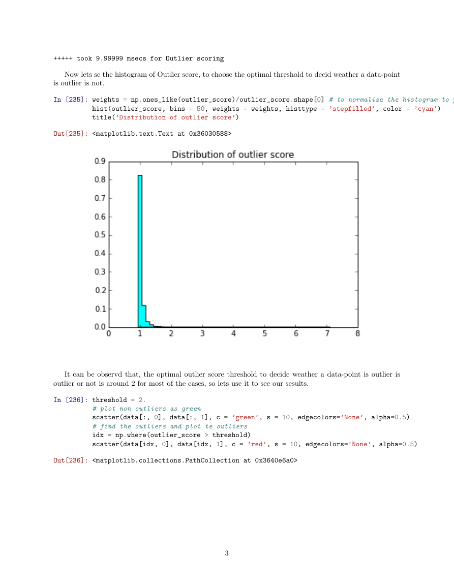
It can be observd that, the optimal outlier score threshold to decide weather a data-point is outlier is
outlier or not is around 2 for most of the cases, so lets use it to see our sesults.
In [236]: threshold = 2.
# plot non outliers as green
scatter(data[:, 0], data[:, 1], c = ’green’, s = 10, edgecolors=’None’, alpha=0.5)
# find the outliers and plot te outliers
idx = np.where(outlier_score > threshold)
scatter(data[idx, 0], data[idx, 1], c = ’red’, s = 10, edgecolors=’None’, alpha=0.5)
Out[236]:
3
�
We have seen the results of LOF with naive approachfor KNN queries. Now lets see optimisations with
KD-Trees.
Using KD Trees KD-Trees insertion and KNN query.
In [239]: from sklearn.neighbors import KDTree as Tree
tic = time.time()
BT = Tree(data, leaf_size=5, p=2)
# Query for k nearest, k + 1 because one of the returnee is self
dx, idx_knn = BT.query(data[:, :], k = k + 1)
print ’++ took %g msecs for Tree KNN Querying’ %
((time.time() - tic)* 1000)
++ took 122 msecs for Tree KNN Querying
LRD computation.
In [240]: tic = time.time()
dx, idx_knn = dx[:, 1:], idx_knn[:, 1:]
# get the radius for each point in dataset
# radius is the distance of kth nearest point for each point in dataset
radius = dx[:, -1]
# calculate the local reachability density
LRD = np.mean(np.maximum(dx, radius[idx_knn]), axis = 1)
print ’++ took %g msecs for LRD computation’ %
((time.time() - tic)* 1000)
++ took 8.99982 msecs for LRD computation
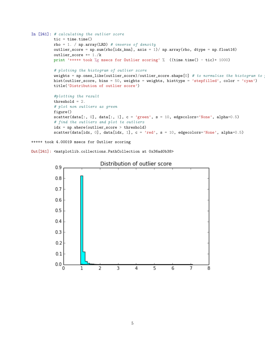
Now, rest is same, so, i’m just replicating the rsult for completion.
4
�
In [241]: # calculating the outlier score
tic = time.time()
rho = 1. / np.array(LRD) # inverse of density
outlier_score = np.sum(rho[idx_knn], axis = 1)/ np.array(rho, dtype = np.float16)
outlier_score *= 1./k
print ’+++++ took %g msecs for Outlier scoring’ %
((time.time() - tic)* 1000)
# plotiing the histogram of outlier score
weights = np.ones_like(outlier_score)/outlier_score.shape[0] # to normalize the histogram to probability plot
hist(outlier_score, bins = 50, weights = weights, histtype = ’stepfilled’, color = ’cyan’)
title(’Distribution of outlier score’)
#plotting the result
threshold = 2.
# plot non outliers as green
figure()
scatter(data[:, 0], data[:, 1], c = ’green’, s = 10, edgecolors=’None’, alpha=0.5)
# find the outliers and plot te outliers
idx = np.where(outlier_score > threshold)
scatter(data[idx, 0], data[idx, 1], c = ’red’, s = 10, edgecolors=’None’, alpha=0.5)
+++++ took 4.00019 msecs for Outlier scoring
Out[241]:
5
�
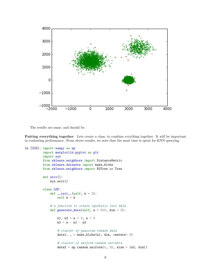
The results are same, and should be.
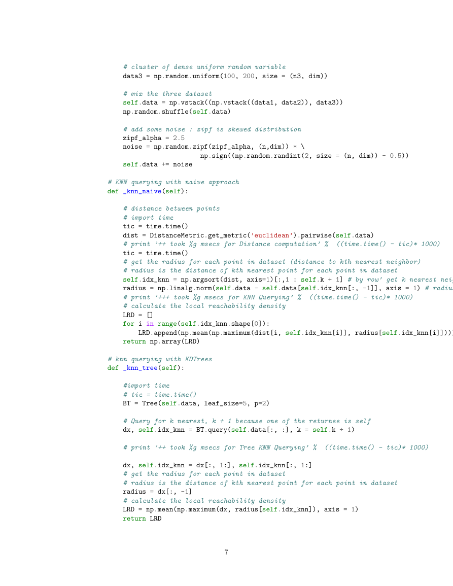
Putting everything together Lets create a class, to combine evrything together. It will be important
in evaluating performance. From above results, we note that the most time is spent for KNN querying.
In [225]: import numpy as np
import matplotlib.pyplot as plt
import sys
from sklearn.neighbors import DistanceMetric
from sklearn.datasets import make_blobs
from sklearn.neighbors import KDTree as Tree
def exit():
sys.exit()
class LOF:
def __init__(self, k = 3):
self.k = k
# a function to create synthetic test data
def generate_data(self, n = 500, dim = 3):
n1, n2 = n / 3, n / 5
n3 = n - n1 - n2
# cluster of gaussian random data
data1, _ = make_blobs(n1, dim, centers= 3)
# cluster of uniform random variable
data2 = np.random.uniform(0, 25, size = (n2, dim))
6
�
# cluster of dense uniform random variable
data3 = np.random.uniform(100, 200, size = (n3, dim))
# mix the three dataset
self.data = np.vstack((np.vstack((data1, data2)), data3))
np.random.shuffle(self.data)
# add some noise : zipf is skewed distribution
zipf_alpha = 2.5
noise = np.random.zipf(zipf_alpha, (n,dim)) * \
np.sign((np.random.randint(2, size = (n, dim)) - 0.5))
self.data += noise
# KNN querying with naive approach
def _knn_naive(self):
# distance between points
# import time
tic = time.time()
dist = DistanceMetric.get_metric(’euclidean’).pairwise(self.data)
# print ’++ took %g msecs for Distance computation’ %
tic = time.time()
# get the radius for each point in dataset (distance to kth nearest neighbor)
# radius is the distance of kth nearest point for each point in dataset
self.idx_knn = np.argsort(dist, axis=1)[:,1 : self.k + 1] # by row’ get k nearest neighbour
radius = np.linalg.norm(self.data - self.data[self.idx_knn[:, -1]], axis = 1) # radius
# print ’+++ took %g msecs for KNN Querying’ %
# calculate the local reachability density
LRD = []
for i in range(self.idx_knn.shape[0]):
((time.time() - tic)* 1000)
((time.time() - tic)* 1000)
LRD.append(np.mean(np.maximum(dist[i, self.idx_knn[i]], radius[self.idx_knn[i]])))
return np.array(LRD)
# knn querying with KDTrees
def _knn_tree(self):
#import time
# tic = time.time()
BT = Tree(self.data, leaf_size=5, p=2)
# Query for k nearest, k + 1 because one of the returnee is self
dx, self.idx_knn = BT.query(self.data[:, :], k = self.k + 1)
# print ’++ took %g msecs for Tree KNN Querying’ %
((time.time() - tic)* 1000)
dx, self.idx_knn = dx[:, 1:], self.idx_knn[:, 1:]
# get the radius for each point in dataset
# radius is the distance of kth nearest point for each point in dataset
radius = dx[:, -1]
# calculate the local reachability density
LRD = np.mean(np.maximum(dx, radius[self.idx_knn]), axis = 1)
return LRD
7
�
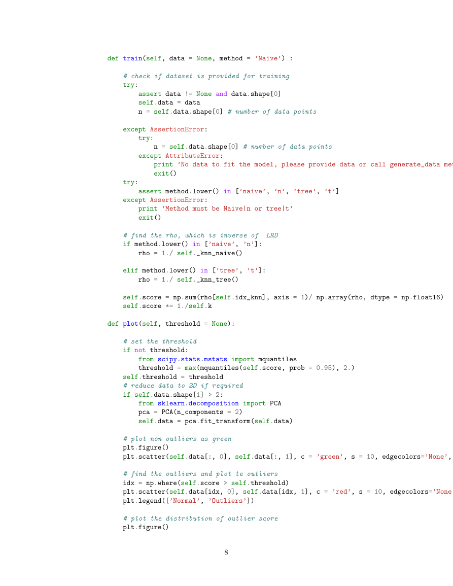
def train(self, data = None, method = ’Naive’) :
# check if dataset is provided for training
try:
assert data != None and data.shape[0]
self.data = data
n = self.data.shape[0] # number of data points
except AssertionError:
try:
n = self.data.shape[0] # number of data points
except AttributeError:
print ’No data to fit the model, please provide data or call generate_data method’
exit()
try:
assert method.lower() in [’naive’, ’n’, ’tree’, ’t’]
except AssertionError:
print ’Method must be Naive|n or tree|t’
exit()
# find the rho, which is inverse of
if method.lower() in [’naive’, ’n’]:
LRD
rho = 1./ self._knn_naive()
elif method.lower() in [’tree’, ’t’]:
rho = 1./ self._knn_tree()
self.score = np.sum(rho[self.idx_knn], axis = 1)/ np.array(rho, dtype = np.float16)
self.score *= 1./self.k
def plot(self, threshold = None):
# set the threshold
if not threshold:
from scipy.stats.mstats import mquantiles
threshold = max(mquantiles(self.score, prob = 0.95), 2.)
self.threshold = threshold
# reduce data to 2D if required
if self.data.shape[1] > 2:
from sklearn.decomposition import PCA
pca = PCA(n_components = 2)
self.data = pca.fit_transform(self.data)
# plot non outliers as green
plt.figure()
plt.scatter(self.data[:, 0], self.data[:, 1], c = ’green’, s = 10, edgecolors=’None’, alpha=0.5)
# find the outliers and plot te outliers
idx = np.where(self.score > self.threshold)
plt.scatter(self.data[idx, 0], self.data[idx, 1], c = ’red’, s = 10, edgecolors=’None’, alpha=0.5)
plt.legend([’Normal’, ’Outliers’])
# plot the distribution of outlier score
plt.figure()
8
�




 2023年江西萍乡中考道德与法治真题及答案.doc
 2012年重庆南川中考生物真题及答案.doc
 2013年江西师范大学地理学综合及文艺理论基础考研真题.doc
 2020年四川甘孜小升初语文真题及答案I卷.doc
 2020年注册岩土工程师专业基础考试真题及答案.doc
 2023-2024学年福建省厦门市九年级上学期数学月考试题及答案.doc
 2021-2022学年辽宁省沈阳市大东区九年级上学期语文期末试题及答案.doc
 2022-2023学年北京东城区初三第一学期物理期末试卷及答案.doc
 2018上半年江西教师资格初中地理学科知识与教学能力真题及答案.doc
 2012年河北国家公务员申论考试真题及答案-省级.doc
 2020-2021学年江苏省扬州市江都区邵樊片九年级上学期数学第一次质量检测试题及答案.doc
 2022下半年黑龙江教师资格证中学综合素质真题及答案.doc