Date of publication xxxx 00, 0000, date of current version xxxx 00, 0000.
Digital Object Identifier 10.1109/ACCESS.2018.DOI
Effective Combination of DenseNet and
BiLSTM for Keyword Spotting
Mengjun Zeng1,Nanfeng Xiao1
1School of Computer Science and Engineering, South China University of Technology, Guangzhou 510006, China
Corresponding author: Mengjun Zeng (e-mail: bob.zeng@outlook.com).
This work was supported by the National Natural Science Foundation of China under Grant [No. 61573145], the Public Research and
Capacity Building of Guangdong Province under Grant [No. 2014B010104001] and the Basic and Applied Basic Research of Guangdong
Province under Grant [No. 2015A03030 8018]
ABSTRACT Keyword spotting (KWS) is a major component of human-computer interaction for smart
on-device terminals and service robots, the purpose of which is to maximize the detection accuracy while
keeping footprint size small. In this paper, based on the powerful ability of DenseNet on extracting local
feature-maps, we propose a new network architecture (DenseNet-BiLSTM) for KWS. In our DenseNet-
BiLSTM, DenseNet is primarily applied to obtain local features, while BiLSTM is used to grab time series
features. In general, DenseNet is used in computer vision tasks, and it may corrupt contextual information
for speech audios. In order to make DenseNet suitable for KWS, we propose a variant DenseNet, called
DenseNet-Speech, which removes the pool on the time dimension in transition layers to preserve speech
time series information. Additionally, our DenseNet-Speech uses less dense blocks and filters to keep the
model small, thereby reducing time consumption for mobile devices. Experimental results show that feature-
maps from DenseNet-Speech maintain time series information well. Our method outperforms the state-of-
the-art methods in terms of accuracy on Google Speech Commands dataset. DenseNet-BiLSTM is able to
achieve the accuracy of 96.6% for the 20-commands recognition task with 223K trainable parameters.
INDEX TERMS keyword spotting, speech recognition, DenseNet, long short-term memory, attention
mechanism
I. INTRODUCTION
H UMAN-COMPUTER interaction is an important part
of artificial intelligence. In the financial fields, special
speech commands can help customers make use of verbal
orders to buy or sell shares, where customers are required
to reply “Yes” or “No” in response to a buy or sell request.
Using special speech commands to wake up a mobile phone
is widely applied nowadays, such as “Hey Siri” on Apple
Devices and ”Okay/Hey Google” [1] on Google Home. It is
also utilized to control industrial and service robots to move
right and left, or to start and stop work, or to do other specific
actions. The technology of detecting a relatively small set of
predefined keywords in a stream of user utterances is called
keyword spotting (KWS). For on-device, the KWS module
should have a high recall rate and a low false alarm. For
industrial and service robots, the speech commands must be
recognized well as much as possible, ensuring the robots
do not do wrong actions. Therefore, for KWS, it is very
important to obtain a good accuracy of speech command
recognition. In addition, the KWS module should also be
small enough to be suitable for mobile devices that may
have low power and performance-limited. We utilize the
number of trainable parameters in the model to measure
the module size. Accordingly, the core goal of KWS is to
improve accuracy while maintaining a reasonable number of
trainable parameters.
Recently, end-to-end models have become popular for
KWS [2]. Convolutional neural network (CNN) [3], [4], deep
neural network (DNN) [5] and residual network (ResNet)
[6] are explored for KWS. One disadvantage of CNN and
ResNet is that they cannot get the long term dependency on
speech audios well. Recurrent neural network (RNN) is also
studied for KWS [7], [8]. A potential limitation of RNN is
that it directly models on the input features without learning
local structure between successive time series and frequency
steps. A few works combined CNN and RNN to improve the
accuracy of KWS, such as convolutional recurrent neural net-
works (CRNN) [9] and gated convolutional long short-term
memory (LSTM) [10], which achieved better performance
than that of using CNN or RNN only.
VOLUME 4, 2016
1
�
M. Zeng et al.: Effective Combination of DenseNet and BiLSTM for Keyword Spotting
II. RELATED WORK
CNN architecture gains significant improvement for KWS
[3]. In [15], audio recognition problems are converted to the
domain of image classification, and achieved good results.
When CNN becomes deeper, it suffers from the problem
of gradient vanishing, which means the gradient can not be
conducted to the front layers well. ResNet [6] is proposed
to solve this problem, which introduces shortcut connections
of F (x) + x, and can skip one or more layers. Inspired by
the shortcut connections in ResNet, DenseNet is proposed
to maximum information flow between layers in CNNs.
DenseNet passes feature-maps to all its subsequent layers
[11], which can transport more information to latter layers
with fewer parameters than ResNet or other deep CNNs. The
significant improvements for recognition task on CIFAR-
10, CIFAR-100, SVHN and ImageNet [11] indicate that
DenseNet is more effective at extracting local feature-maps
than conventional CNNs. In [16], DenseNet is combined with
transfer learning for speech command recognition, and gets
the accuracy of 85.52%.
LSTM [17] is a type of RNN architecture, which is de-
veloped to deal with the problems of exploding and van-
ishing gradient. It can memorize the value over any time
interval and control the information flowing into the latter
sequence. LSTM with connectionist temporal classification
(CTC) outperforms the deep neural network (DNN) and hid-
den Markov model (HMM) for KWS [7]. BiLSTM can im-
port information from the past and future of the current time,
which introduces more contextual information and achieves
great success on automatic speech recognition. Graves et al.
[18] proposed the combination of deep BiLSTM and HMM,
and its performance is superior to GMM and depth neural
network benchmark on a subset of the Wall Street Journal
corpus. For keyword spotting problem, the model, which uses
only BiLSTM, defeats an HMM-based speech recognizer by
a large margin [19].
There are also many related works about combining CNN
and RNN for KWS. Arik et al. [9] proposed a network ar-
chitecture consisting of one layer CNN and two-layer RNNs
with a total parameter of 229K. Another model [10], which
uses gated CNN with LSTM, has one layer CNN, two layers
Gated CNN and one layer BiLSTM (C-1-G-2-Blstm). The
C-1-G-2-Blstm has a total number of 150K trainable param-
eters, and gains a higher accuracy than Transfer Learning
Network [16] by 6.4% on Google Speech Commands dataset.
Inspired by the success of using CNN along with RNN, and
the powerful ability of extracting local features of DenseNet,
we propose a method of combining DenseNet and BiLSTM
to achieve better performance for KWS.
Besides, the attention mechanism [20], [21] allows neural
networks to focus on different parts of inputs. The attention-
based models achieve better accuracy for KWS. An attention-
based model gets great success in Google Speech Commands
dataset [12]. In [22], an attention-based end-to-end model
is introduced for small-footprint KWS, which defeats deep
KWS system. To get better performance, we also import
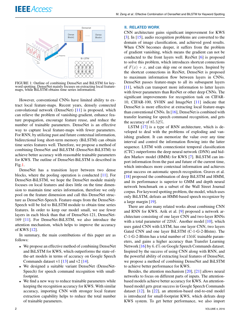
FIGURE 1: Outline of combining DenseNet and BiLSTM for key-
word spotting. DenseNet mainly focuses on extracting local feature-
maps, while BiLSTM obtains time series information.
However, conventional CNNs have limited ability to ex-
tract local feature-maps. Recent years, densely connected
convolutional network (DenseNet) [11] is proposed, which
can relieve the problem of vanishing-gradient, enhance fea-
ture propagation, encourage feature reuse, and reduce the
number of trainable parameters. DenseNet is an effective
way to capture local feature-maps with fewer parameters.
For RNN, by utilizing past and future contextual information,
bidirectional long short-term memory (BiLSTM) can obtain
time series features well. Therefore, we propose a method of
combining DenseNet and BiLSTM (DenseNet-BiLSTM) to
achieve better accuracy with reasonable trainable parameters
for KWS. The outline of DenseNet-BiLSTM is described in
Fig.1.
DenseNet has a transition layer between two dense
blocks, where the pooling operation is conducted [11]. For
DenseNet-BiLSTM, we hope the DenseNet module mainly
focuses on local features and does little on the time dimen-
sion to maintain time series information, therefore we only
pool on the feature dimension and call this DenseNet struc-
ture as DenseNet-Speech. Feature-maps from the DenseNet-
Speech will be fed to BiLSTM module to obtain time series
features. In order to keep our model small, we use fewer
layers in each block than that of DenseNet-121, DenseNet-
169 [11]. For DenseNet-BiLSTM, we also introduce the
attention mechanism, which helps to improve the accuracy
of KWS [12].
In summary, the main contributions of this paper are as
follows:
• We propose an effective method of combining DenseNet
and BiLSTM for KWS, which outperforms the state-of-
the-art models in terms of accuracy on Google Speech
Commands dataset v1 [13] and v2 [14].
• We designed a suitable variant DenseNet (DenseNet-
Speech) for speech command recognition with small-
footprint.
• We find a new way to reduce trainable parameters while
keeping the recognition accuracy for KWS. With similar
accuracy, importing CNN with stronger local feature
extraction capability helps to reduce the total number
of trainable parameters.
2
VOLUME 4, 2016
�
M. Zeng et al.: Effective Combination of DenseNet and BiLSTM for Keyword Spotting
attention mechanism to our model.
III. METHODS
A. AUDIO FEATURE EXTRACTION
Spectral representation is the basis of digital signal process
in general. The Mel frequency scale is usually used to
represent audio signals. We use Mel-scale spectrogram [23]
to preprocess speech audios. For every utterance, Mel-scale
spectrogram is computed using an 80-band Mel scale, 1024
discrete Fourier transform points and a hop size of 128.
All frames of each utterance are stacked to form a two-
dimensional vector. The Mel-spectrogram is then converted
to dB-scaled spectrogram for further processing.
B. MODEL ARCHITECTURE
C. DENSENET-SPEECH
For DenseNet, features are passed to all the subsequent layers
in each dense block [11]. Therefore, the l − th layer gets the
feature-maps from all preceding layers as input:
xl = H([x0 : x1 : ... : xl−1])
(1)
where, [x0 : x1 : ... : xl−1] refers to the concatenation of the
feature-maps produced in layers 0, . . . , l − 1.
In general, there are several dense blocks, transition layers
and one classification layer in DenseNet [11]. At the begin-
ning of DenseNet-121, DenseNet-169 [11], a convolution of
a 7×7 kernel with stride 2×2 is used. But in the same position
of our DenseNet-Speech, we only perform a convolution
operation along the time dimension to get the basic feature-
maps of the time series. The convolution has a kernel of 5×1,
without any pooling operation.
There are four dense blocks, and the number of layers in
each dense block is different in DenseNet-121, DenseNet-
169 [11]. In order to keep the trainable parameters small, we
use fewer dense blocks in DenseNet-Speech. In each dense
block, the number of layers is set to be the same.
TABLE 1: DenseNet-Speech Architecture for Google Speech Com-
mands dataset. We set the number of dense blocks to 3 as the
example. The growth rate k=10. Each ‘conv’ shown on the table
corresponds the sequence BN-ReLU-Conv. The number after ‘conv’
is the output channels. The batch size is ignored in the output size.
DenseNet-Speech (k=10)
Layers
Convolution
Pooling
Dense Block(1)
Transition
Layer(1)
Dense Block(2)
Transition
Layer(2)
Dense Block(3)
Reshape Layer
Output Size
126 × 80 × 10
53 × 40 × 10
53 × 40 × 10
53 × 40 × 10
53 × 20 × 10
53 × 20 × 10
53 × 20 × 10
53 × 10 × 10
53 × 10 × 10
53 × 10 × 1
53 × 10
5 × 1 conv(10)
2 × 2 average
pooling, stride 2 × 2
1 × 1 conv(40)
× 6
3 × 3 conv(10)
1 × 1 conv(10)
1 × 2, average
pooling, stride 1 × 2
1 × 1 conv(40)
× 6
3 × 3 conv(10)
1 × 1 conv(10)
1 × 2, average
pooling, stride 1 × 2
1 × 1 conv(40)
× 6
3 × 3 conv(10)
3 × 3 conv(1)
reshape
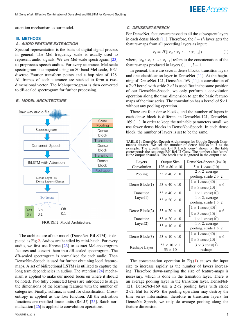
FIGURE 2: Model Architecture.
The architecture of our model (DenseNet-BiLSTM), is de-
picted as Fig.2. Audios are handled by mini-batch. For every
audio, we first use librosa [23] to extract Mel-spectrogram
features and convert them into dB-scaled spectrogram. The
dB-scaled spectrogram is normalized for each audio. Then
DenseNet-Speech is used for further obtaining local feature-
maps. A set of bidirectional LSTMs is utilized to capture the
long term dependencies in audios. The attention [24] mecha-
nism is applied to make our model focus on where it should
be noted. Two fully connected layers are introduced to align
the dimensions of the learning features with the number of
categories. Finally, softmax is used for classification. Cross-
entropy is applied as the loss function. All the activation
functions are rectified linear units (ReLU) [25]. Batch nor-
malization [26] is applied to convolution operations.
VOLUME 4, 2016
The concatenation operation in Eq.(1) causes the input
size to increase rapidly as the number of layers increas-
ing. Therefore down-sampling the size of feature-maps is
necessary, which is done in the transition layer. There is
an average pooling layer in the transition layer. DenseNet-
121, DenseNet-169 use a 2×2 pooling layer with stride
2×2. But for KWS, the pooling operation may destroy the
time series information, therefore in transition layers for
DenseNet-Speech, we only do average pooling along the
feature dimension.
3
�
In the classification layer for the DenseNet model in [11],
there is a global average pooling layer and a fully connected
layer. We discard the global average pooling layer in our
DenseNet-Speech, and use a reshape layer instead of the fully
connected layer. The reshape layer adapts the dimensions of
the feature-maps to BiLSTM layers.
For Google Speech Commands dataset, the size of dB-
scaled spectrogram of an audio is 126×80. A global average
pooling with stride 2×2 in the beginning, is introduced to
reduce parameters. The architecture of DenseNet-Speech for
Google Speech Commands dataset is detailed in Table 1.
D. BILSTM WITH ATTENTION
LSTM is a recurrent model, in which the current time pre-
diction depends on all past time inputs. For each layer, the
LSTM processes at time t by computing
ft = σg(Wf xt + Uf ht−1 + bf )
it = σg(Wixt + Uiht−1 + bi)
ot = σg(Woxt + Uoht−1 + bo)
ct = ftct−1 + itσc(Wcxt + Ucht−1 + bc)
ht = otσh(ct)
(2)
(3)
(4)
(5)
(6)
where, σg is sigmoid function, σc and σh is hyperbolic
tangent function, f, i, o are gates, c is the internal cell states,
h is the hidden states.
LSTM only uses past information. BiLSTM can also take
advantage of future information. In each BiLSTM layer, there
are a forward pass and a backward pass. The forward pass
gets feature-maps according to Eq.(2)-Eq.(6), whereas the
backward pass does the opposite by changing all t − 1 to
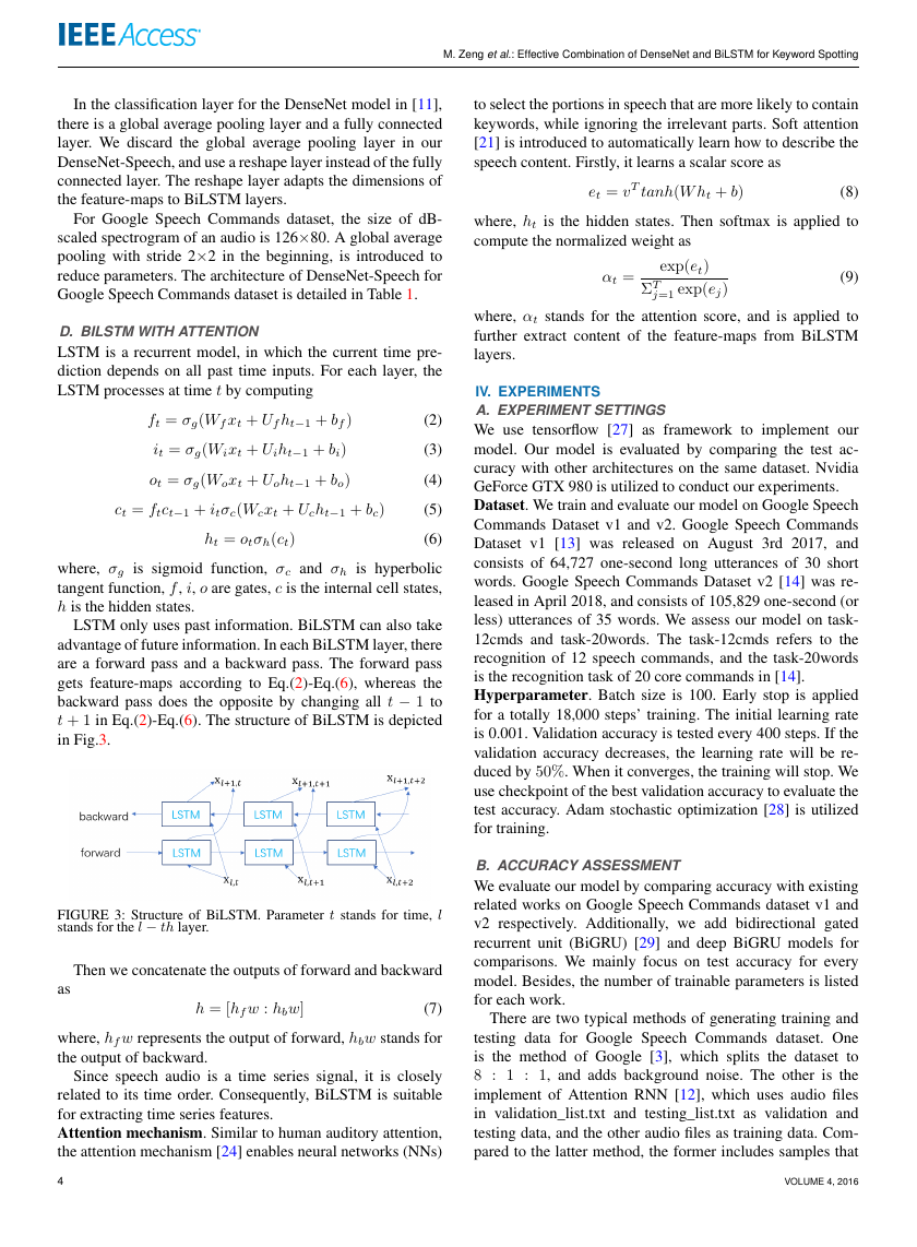
t + 1 in Eq.(2)-Eq.(6). The structure of BiLSTM is depicted
in Fig.3.
FIGURE 3: Structure of BiLSTM. Parameter t stands for time, l
stands for the l − th layer.
as
Then we concatenate the outputs of forward and backward
h = [hf w : hbw]
(7)
where, hf w represents the output of forward, hbw stands for
the output of backward.
Since speech audio is a time series signal, it is closely
related to its time order. Consequently, BiLSTM is suitable
for extracting time series features.
Attention mechanism. Similar to human auditory attention,
the attention mechanism [24] enables neural networks (NNs)
4
M. Zeng et al.: Effective Combination of DenseNet and BiLSTM for Keyword Spotting
to select the portions in speech that are more likely to contain
keywords, while ignoring the irrelevant parts. Soft attention
[21] is introduced to automatically learn how to describe the
speech content. Firstly, it learns a scalar score as
et = vT tanh(W ht + b)
(8)
where, ht is the hidden states. Then softmax is applied to
compute the normalized weight as
αt =
exp(et)
j=1 exp(ej)
ΣT
(9)
where, αt stands for the attention score, and is applied to
further extract content of the feature-maps from BiLSTM
layers.
IV. EXPERIMENTS
A. EXPERIMENT SETTINGS
We use tensorflow [27] as framework to implement our
model. Our model is evaluated by comparing the test ac-
curacy with other architectures on the same dataset. Nvidia
GeForce GTX 980 is utilized to conduct our experiments.
Dataset. We train and evaluate our model on Google Speech
Commands Dataset v1 and v2. Google Speech Commands
Dataset v1 [13] was released on August 3rd 2017, and
consists of 64,727 one-second long utterances of 30 short
words. Google Speech Commands Dataset v2 [14] was re-
leased in April 2018, and consists of 105,829 one-second (or
less) utterances of 35 words. We assess our model on task-
12cmds and task-20words. The task-12cmds refers to the
recognition of 12 speech commands, and the task-20words
is the recognition task of 20 core commands in [14].
Hyperparameter. Batch size is 100. Early stop is applied
for a totally 18,000 steps’ training. The initial learning rate
is 0.001. Validation accuracy is tested every 400 steps. If the
validation accuracy decreases, the learning rate will be re-
duced by 50%. When it converges, the training will stop. We
use checkpoint of the best validation accuracy to evaluate the
test accuracy. Adam stochastic optimization [28] is utilized
for training.
B. ACCURACY ASSESSMENT
We evaluate our model by comparing accuracy with existing
related works on Google Speech Commands dataset v1 and
v2 respectively. Additionally, we add bidirectional gated
recurrent unit (BiGRU) [29] and deep BiGRU models for
comparisons. We mainly focus on test accuracy for every
model. Besides, the number of trainable parameters is listed
for each work.
There are two typical methods of generating training and
testing data for Google Speech Commands dataset. One
is the method of Google [3], which splits the dataset to
8 : 1 : 1, and adds background noise. The other is the
implement of Attention RNN [12], which uses audio files
in validation_list.txt and testing_list.txt as validation and
testing data, and the other audio files as training data. Com-
pared to the latter method, the former includes samples that
VOLUME 4, 2016
�
M. Zeng et al.: Effective Combination of DenseNet and BiLSTM for Keyword Spotting
only have background noise in testing data. In this section,
DenseNet-BiLSTM includes 3 layers of dense blocks and
trains following the implement of Attention RNN, while
DenseN et − BiLST M has 2 layers of dense blocks and
trains following Google’s implement.
TABLE 2: Accuracy on Google Speech Commands dataset v1.
ConvNet comes from [3]. tpool2 results from [30]. Res26, res15
results from [6]. DS-CNN results from [31]. C-1-G-2-Blstm results
from [10]. Attention RNN results from [12]. TDNN results from
[32]. HD-CNN comes from [33]. BiLSTM-i (BiGRU-i) refers to
the model which has i layers’ BiLSTM (BiGRU). DenseNet-BiGRU
stands for the model which combines DenseNet and BiGRU. Res15,
Res26, TDNN, DS-CNN follows Google’s implement. C-1-G-2-
Blstm splits dataset as the way of Attention RNN. ConvNet,
BiLSTM-2, BiLSTM-5, BiGRU-2, BiGRU-5, BiGRU-8 and HD-
CNN are trained by us.
Model
Accuracy(%)
(12cmds)
Accuracy(%)
(20words)
Trainable
Parameters
increases the accuracy by 8.4%. Compared to the Attention
RNN [12], our DenseNet-BiLSTM reduces WER by 16% for
task-12cmds, 25% for task-20words with 25% more trainable
parameters. As to RENA [34], our model reduces WER
by 35.7% with 56% more trainable parameters. Therefore
our model makes a good job on Google Speech Commands
dataset v2.
Table 2 and Table 3 show that our model achieves a
new state-of-the-art performance on Google Speech Com-
mands dataset v1 and v2 for task-12cmds and task-20words
with reasonable trainable parameters. Our model reduces the
WER significantly, gains great improvements in the accuracy
of speech command recognition tasks.
ConvNet
tpool2
BiLSTM-2
TDNN
BiLSTM-5
BiGRU-2
Res26
DS-CNN
HD-CNN
BiGRU-8
BiGRU-5
Res15
DenseNet-BiGRU
DenseN et − BiLST M
C-1-G-2-Blstm
Attention RNN
DenseNet-BiLSTM
90.5
91.97
93.6
94.3
94.5
94.7
95.2
95.4
95.6
95.7
95.8
95.8
96.1
96.2
N/A
95.6
97.5
N/A
N/A
N/A
N/A
N/A
N/A
N/A
N/A
N/A
N/A
N/A
N/A
N/A
N/A
90.9
94.1
95.7
926K
1.09M
190K
N/A
486K
147K
438K
497K
40M
591K
369K
238K
188k
223K
150K
202K
250K
For Google Speech Commands dataset v1, Table 2 shows
that our model achieves the best performance for the two
tasks. Compared to BiGRU-5 and Res15 [6] for task-12cmds,
our model reduced the word error rate (WER) by 9.5% with
fewer parameters. Although BiGRU-based models perform
better than BiLSTM-based models, DenseNet-BiLSTM gets
a little higher accuracy than DenseNet-BiGRU. As to the
Attention RNN [12], with the same method of generating
training and test data, our model reduces the WER by 40%
for task-12cmds, and by 27% for task-20words. The number
of trainable parameters of our model is 25% more than the
Attention RNN. Therefore, our model achieves a new state-
of-the-art performance on Google Speech Commands dataset
v1 with reasonable trainable parameters.
TABLE 3: Accuracy on Google Speech Commands dataset v2.
ConvNet results from [14]. Attention RNN results from [12]. RENA
results from [34]. RENA follows Google’s implement.
Model
Accuracy(%)
(12cmds)
Accuracy(%)
(20words)
Trainable
Parameters
ConvNet
RENA
DenseN et − BiLST M
Attention RNN
DenseNet-BiLSTM
N/A
95.8
97.3
96.9
97.4
88.2
N/A
96.6
94.5
95.9
N/A
143K
223K
202K
250K
Table 3 illustrates the results on Google Speech Com-
mands dataset v2. In contrast to ConvNet [14], our model
VOLUME 4, 2016
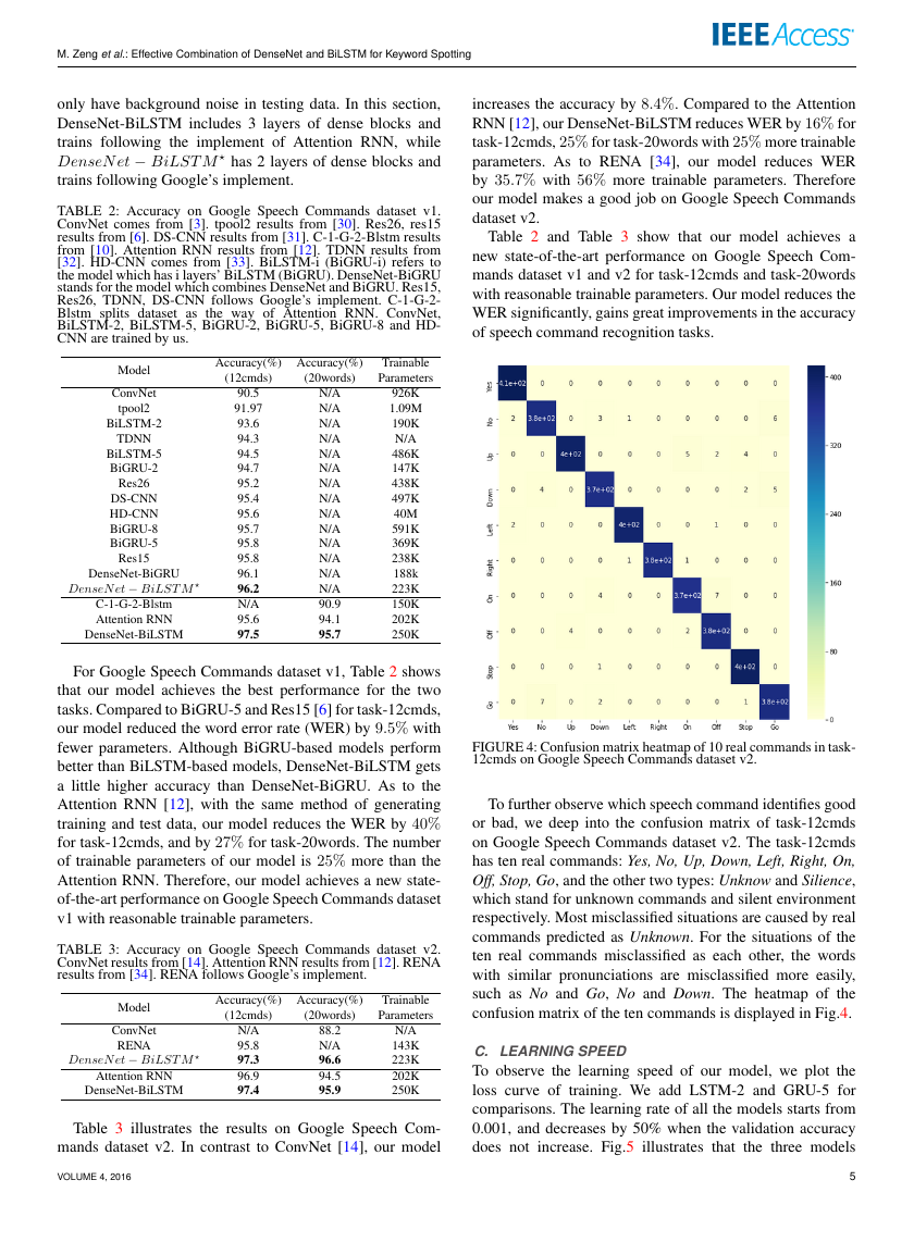
FIGURE 4: Confusion matrix heatmap of 10 real commands in task-
12cmds on Google Speech Commands dataset v2.
To further observe which speech command identifies good
or bad, we deep into the confusion matrix of task-12cmds
on Google Speech Commands dataset v2. The task-12cmds
has ten real commands: Yes, No, Up, Down, Left, Right, On,
Off, Stop, Go, and the other two types: Unknow and Silience,
which stand for unknown commands and silent environment
respectively. Most misclassified situations are caused by real
commands predicted as Unknown. For the situations of the
ten real commands misclassified as each other, the words
with similar pronunciations are misclassified more easily,
such as No and Go, No and Down. The heatmap of the
confusion matrix of the ten commands is displayed in Fig.4.
C. LEARNING SPEED
To observe the learning speed of our model, we plot the
loss curve of training. We add LSTM-2 and GRU-5 for
comparisons. The learning rate of all the models starts from
0.001, and decreases by 50% when the validation accuracy
does not increase. Fig.5 illustrates that the three models
5
�
M. Zeng et al.: Effective Combination of DenseNet and BiLSTM for Keyword Spotting
IMPACT OF DIFFERENT DENSENET-SPEECH
E.
There are many hyperparameters for DenseNet-Speech, such
as the growth rate, the number of dense blocks, CNN kernels
and so on. Here we discuss the impact of different growth
rates and dense block numbers.
Impact of the grow rate. For each dense block, the size of
input feature-maps of l − th layer can be calculated by
f ll = f l0 + (l − 1) ∗ k
(10)
where, f l0 is the size of input features-maps of the first layer
in a dense block, k is the growth rate. With l increasing, f ll
increases heavily. Therefore the growth rate is an important
hyperparameter. We set the growth rate to different values
to assess the impact of the growth rate for our model. The
number of dense blocks is set to three. We evaluate on the
task-12cmds using Google Speech Commands Dataset v1.
TABLE 4: Impact of the grow rate (k).
Grow rate(k) Accuracy(%) Trainable Parameters
5
10
15
97.4
97.5
97.4
179K
250K
367K
Table 4 demonstrates that as the growth rate increasing, the
number of trainable parameters becomes much larger. When
k=10, the accuracy is the best of the three in the table. The
accuracy does not increase when the growth rate increases
from 10 to 15.
Impact of the number of dense blocks. The number of
dense blocks has a significant influence on the depth of
DenseNet-Speech. More dense blocks require more trainable
parameters. We set the dense block number to different
values to evaluate the impact of dense blocks. The growth
rate is set to 10. We evaluate on Google Speech Commands
dataset v1 for task-12cmds.
TABLE 5: Impact of the number of dense blocks.
FIGURE 5: Learning speed. The smoothingWeight is 0.95. Models
here are all trained and evaluated on Google Speech Commands
dataset v1.
all converge quickly, which owes to the Adam stochastic
optimization [28]. The loss value of our model is the smallest
after convergence.
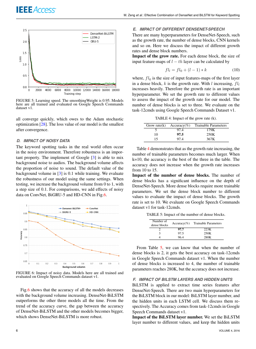
IMPACT OF NOISY DATA
D.
The keyword spotting tasks in the real world often occur
in the noisy environment. Therefore robustness is an impor-
tant property. The implement of Google [3] is able to mix
background noise to audios. The background volume affects
the proportion of noise to sound. The default value of the
background volume in [3] is 0.1 while training. We evaluate
the robustness of our model using the same settings. When
testing, we increase the background volume from 0 to 1, with
a step size of 0.1. For comparisons, we add effects of noisy
data on ConvNet, BiGRU-5 and HD-CNN in Fig.6.
Number of
dense blocks Accuracy(%) Trainable Parameters
223K
250K
280K
2
3
4
97.7
97.5
96.4
FIGURE 6: Impact of noisy data. Models here are all trained and
evaluated on Google Speech Commands dataset v1.
Fig.6 shows that the accuracy of all the models decreases
with the background volume increasing. DenseNet-BiLSTM
outperforms the other three models all the time. From the
trend of the accuracy curve, the gap between the accuracy
of DenseNet-BiLSTM and the other models becomes bigger,
which shows DenseNet-BiLSTM is more robust.
6
From Table 5, we can know that when the number of
dense blocks is 2, it gets the best accuracy on task-12cmds
in Google Speech Commands dataset v1. When the number
of dense blocks is increased to 4, the number of trainable
parameters reaches 280K, but the accuracy does not increase.
IMPACT OF BILSTM LAYERS AND HIDDEN UNITS
F.
BiLSTM is applied to extract
time series features after
DenseNet-Speech. There are two main hyperparameters for
the BiLSTM block in our model: BiLSTM layer number, and
the hidden units in each LSTM cell. We discuss them re-
spectively. The Accuracy comes from task-12cmds in Google
Speech Commands dataset v1.
Impact of the BiLSTM layer number. We set the BiLSTM
layer number to different values, and keep the hidden units
VOLUME 4, 2016
�
M. Zeng et al.: Effective Combination of DenseNet and BiLSTM for Keyword Spotting
(a)
(b)
(c)
(d)
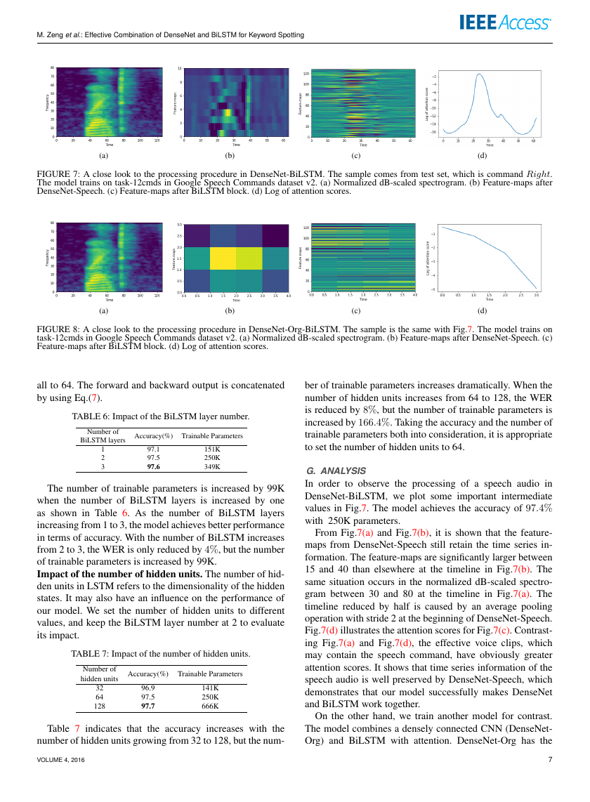
FIGURE 7: A close look to the processing procedure in DenseNet-BiLSTM. The sample comes from test set, which is command Right.
The model trains on task-12cmds in Google Speech Commands dataset v2. (a) Normalized dB-scaled spectrogram. (b) Feature-maps after
DenseNet-Speech. (c) Feature-maps after BiLSTM block. (d) Log of attention scores.
(a)
(b)
(c)
(d)
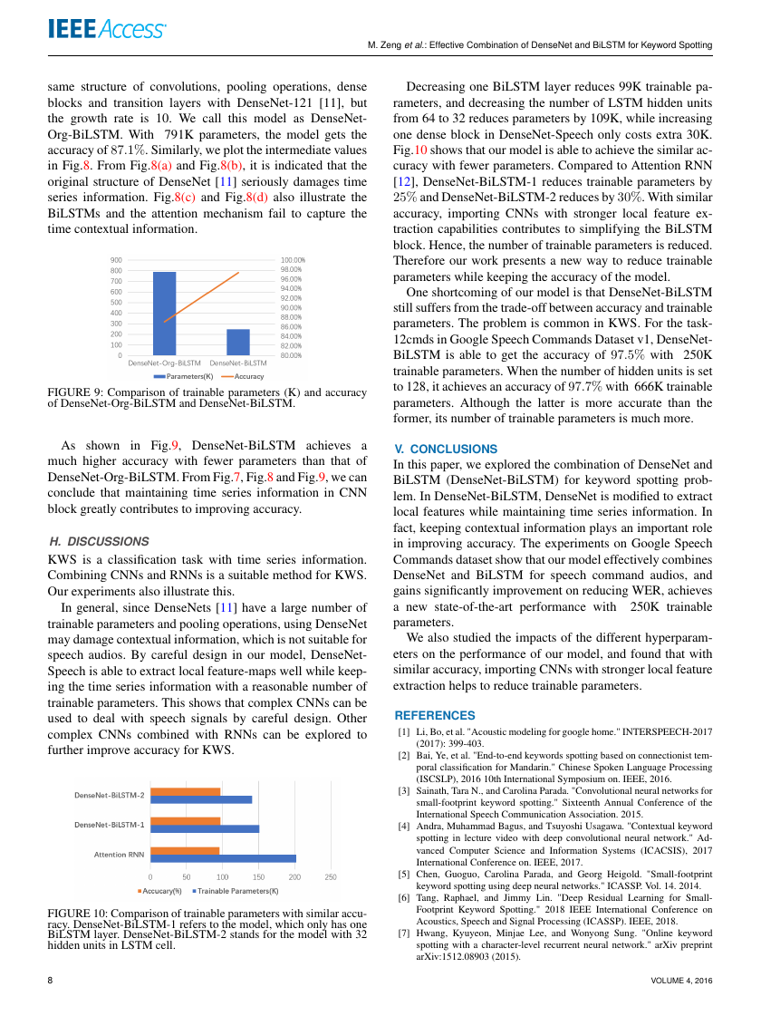
FIGURE 8: A close look to the processing procedure in DenseNet-Org-BiLSTM. The sample is the same with Fig.7. The model trains on
task-12cmds in Google Speech Commands dataset v2. (a) Normalized dB-scaled spectrogram. (b) Feature-maps after DenseNet-Speech. (c)
Feature-maps after BiLSTM block. (d) Log of attention scores.
all to 64. The forward and backward output is concatenated
by using Eq.(7).
TABLE 6: Impact of the BiLSTM layer number.
Number of
BiLSTM layers Accuracy(%) Trainable Parameters
1
2
3
97.1
97.5
97.6
151K
250K
349K
The number of trainable parameters is increased by 99K
when the number of BiLSTM layers is increased by one
as shown in Table 6. As the number of BiLSTM layers
increasing from 1 to 3, the model achieves better performance
in terms of accuracy. With the number of BiLSTM increases
from 2 to 3, the WER is only reduced by 4%, but the number
of trainable parameters is increased by 99K.
Impact of the number of hidden units. The number of hid-
den units in LSTM refers to the dimensionality of the hidden
states. It may also have an influence on the performance of
our model. We set the number of hidden units to different
values, and keep the BiLSTM layer number at 2 to evaluate
its impact.
TABLE 7: Impact of the number of hidden units.
Number of
hidden units Accuracy(%) Trainable Parameters
32
64
128
96.9
97.5
97.7
141K
250K
666K
Table 7 indicates that the accuracy increases with the
number of hidden units growing from 32 to 128, but the num-
VOLUME 4, 2016
ber of trainable parameters increases dramatically. When the
number of hidden units increases from 64 to 128, the WER
is reduced by 8%, but the number of trainable parameters is
increased by 166.4%. Taking the accuracy and the number of
trainable parameters both into consideration, it is appropriate
to set the number of hidden units to 64.
G. ANALYSIS
In order to observe the processing of a speech audio in
DenseNet-BiLSTM, we plot some important intermediate
values in Fig.7. The model achieves the accuracy of 97.4%
with 250K parameters.
From Fig.7(a) and Fig.7(b), it is shown that the feature-
maps from DenseNet-Speech still retain the time series in-
formation. The feature-maps are significantly larger between
15 and 40 than elsewhere at the timeline in Fig.7(b). The
same situation occurs in the normalized dB-scaled spectro-
gram between 30 and 80 at the timeline in Fig.7(a). The
timeline reduced by half is caused by an average pooling
operation with stride 2 at the beginning of DenseNet-Speech.
Fig.7(d) illustrates the attention scores for Fig.7(c). Contrast-
ing Fig.7(a) and Fig.7(d), the effective voice clips, which
may contain the speech command, have obviously greater
attention scores. It shows that time series information of the
speech audio is well preserved by DenseNet-Speech, which
demonstrates that our model successfully makes DenseNet
and BiLSTM work together.
On the other hand, we train another model for contrast.
The model combines a densely connected CNN (DenseNet-
Org) and BiLSTM with attention. DenseNet-Org has the
7
�
same structure of convolutions, pooling operations, dense
blocks and transition layers with DenseNet-121 [11], but
the growth rate is 10. We call this model as DenseNet-
Org-BiLSTM. With 791K parameters, the model gets the
accuracy of 87.1%. Similarly, we plot the intermediate values
in Fig.8. From Fig.8(a) and Fig.8(b), it is indicated that the
original structure of DenseNet [11] seriously damages time
series information. Fig.8(c) and Fig.8(d) also illustrate the
BiLSTMs and the attention mechanism fail to capture the
time contextual information.
FIGURE 9: Comparison of trainable parameters (K) and accuracy
of DenseNet-Org-BiLSTM and DenseNet-BiLSTM.
As
shown in Fig.9, DenseNet-BiLSTM achieves a
much higher accuracy with fewer parameters than that of
DenseNet-Org-BiLSTM. From Fig.7, Fig.8 and Fig.9, we can
conclude that maintaining time series information in CNN
block greatly contributes to improving accuracy.
H. DISCUSSIONS
KWS is a classification task with time series information.
Combining CNNs and RNNs is a suitable method for KWS.
Our experiments also illustrate this.
In general, since DenseNets [11] have a large number of
trainable parameters and pooling operations, using DenseNet
may damage contextual information, which is not suitable for
speech audios. By careful design in our model, DenseNet-
Speech is able to extract local feature-maps well while keep-
ing the time series information with a reasonable number of
trainable parameters. This shows that complex CNNs can be
used to deal with speech signals by careful design. Other
complex CNNs combined with RNNs can be explored to
further improve accuracy for KWS.
FIGURE 10: Comparison of trainable parameters with similar accu-
racy. DenseNet-BiLSTM-1 refers to the model, which only has one
BiLSTM layer. DenseNet-BiLSTM-2 stands for the model with 32
hidden units in LSTM cell.
M. Zeng et al.: Effective Combination of DenseNet and BiLSTM for Keyword Spotting
Decreasing one BiLSTM layer reduces 99K trainable pa-
rameters, and decreasing the number of LSTM hidden units
from 64 to 32 reduces parameters by 109K, while increasing
one dense block in DenseNet-Speech only costs extra 30K.
Fig.10 shows that our model is able to achieve the similar ac-
curacy with fewer parameters. Compared to Attention RNN
[12], DenseNet-BiLSTM-1 reduces trainable parameters by
25% and DenseNet-BiLSTM-2 reduces by 30%. With similar
accuracy, importing CNNs with stronger local feature ex-
traction capabilities contributes to simplifying the BiLSTM
block. Hence, the number of trainable parameters is reduced.
Therefore our work presents a new way to reduce trainable
parameters while keeping the accuracy of the model.
One shortcoming of our model is that DenseNet-BiLSTM
still suffers from the trade-off between accuracy and trainable
parameters. The problem is common in KWS. For the task-
12cmds in Google Speech Commands Dataset v1, DenseNet-
BiLSTM is able to get the accuracy of 97.5% with 250K
trainable parameters. When the number of hidden units is set
to 128, it achieves an accuracy of 97.7% with 666K trainable
parameters. Although the latter is more accurate than the
former, its number of trainable parameters is much more.
V. CONCLUSIONS
In this paper, we explored the combination of DenseNet and
BiLSTM (DenseNet-BiLSTM) for keyword spotting prob-
lem. In DenseNet-BiLSTM, DenseNet is modified to extract
local features while maintaining time series information. In
fact, keeping contextual information plays an important role
in improving accuracy. The experiments on Google Speech
Commands dataset show that our model effectively combines
DenseNet and BiLSTM for speech command audios, and
gains significantly improvement on reducing WER, achieves
a new state-of-the-art performance with
250K trainable
parameters.
We also studied the impacts of the different hyperparam-
eters on the performance of our model, and found that with
similar accuracy, importing CNNs with stronger local feature
extraction helps to reduce trainable parameters.
REFERENCES
[1] Li, Bo, et al. "Acoustic modeling for google home." INTERSPEECH-2017
(2017): 399-403.
[2] Bai, Ye, et al. "End-to-end keywords spotting based on connectionist tem-
poral classification for Mandarin." Chinese Spoken Language Processing
(ISCSLP), 2016 10th International Symposium on. IEEE, 2016.
[3] Sainath, Tara N., and Carolina Parada. "Convolutional neural networks for
small-footprint keyword spotting." Sixteenth Annual Conference of the
International Speech Communication Association. 2015.
[4] Andra, Muhammad Bagus, and Tsuyoshi Usagawa. "Contextual keyword
spotting in lecture video with deep convolutional neural network." Ad-
vanced Computer Science and Information Systems (ICACSIS), 2017
International Conference on. IEEE, 2017.
[5] Chen, Guoguo, Carolina Parada, and Georg Heigold. "Small-footprint
keyword spotting using deep neural networks." ICASSP. Vol. 14. 2014.
[6] Tang, Raphael, and Jimmy Lin. "Deep Residual Learning for Small-
Footprint Keyword Spotting." 2018 IEEE International Conference on
Acoustics, Speech and Signal Processing (ICASSP). IEEE, 2018.
[7] Hwang, Kyuyeon, Minjae Lee, and Wonyong Sung. "Online keyword
spotting with a character-level recurrent neural network." arXiv preprint
arXiv:1512.08903 (2015).
8
VOLUME 4, 2016
�



 2023年江西萍乡中考道德与法治真题及答案.doc
 2012年重庆南川中考生物真题及答案.doc
 2013年江西师范大学地理学综合及文艺理论基础考研真题.doc
 2020年四川甘孜小升初语文真题及答案I卷.doc
 2020年注册岩土工程师专业基础考试真题及答案.doc
 2023-2024学年福建省厦门市九年级上学期数学月考试题及答案.doc
 2021-2022学年辽宁省沈阳市大东区九年级上学期语文期末试题及答案.doc
 2022-2023学年北京东城区初三第一学期物理期末试卷及答案.doc
 2018上半年江西教师资格初中地理学科知识与教学能力真题及答案.doc
 2012年河北国家公务员申论考试真题及答案-省级.doc
 2020-2021学年江苏省扬州市江都区邵樊片九年级上学期数学第一次质量检测试题及答案.doc
 2022下半年黑龙江教师资格证中学综合素质真题及答案.doc