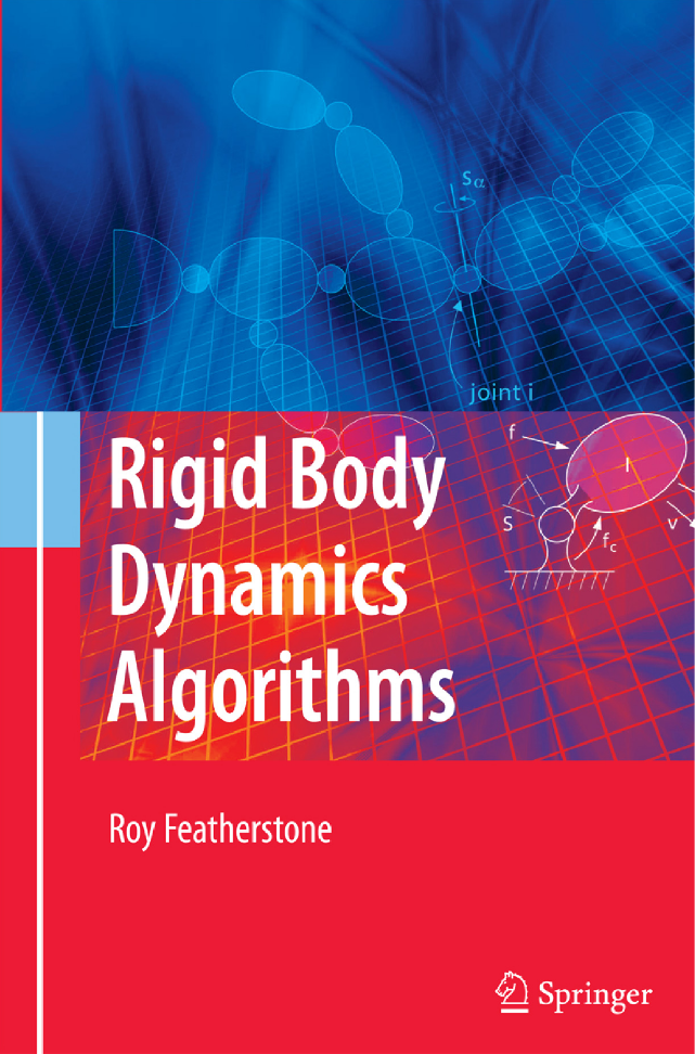
Rigid Body Dynamics Algorithms.pdf-资料库

u013704543-9687940-4744302543452563614.pdf-第1页.png

第1页 / 共276页

u013704543-9687940-4744302543452563614.pdf-第2页.png

第2页 / 共276页

u013704543-9687940-4744302543452563614.pdf-第3页.png

第3页 / 共276页

u013704543-9687940-4744302543452563614.pdf-第4页.png

第4页 / 共276页

u013704543-9687940-4744302543452563614.pdf-第5页.png

第5页 / 共276页

u013704543-9687940-4744302543452563614.pdf-第6页.png

第6页 / 共276页

u013704543-9687940-4744302543452563614.pdf-第7页.png

第7页 / 共276页

u013704543-9687940-4744302543452563614.pdf-第8页.png

第8页 / 共276页

Rigid Body Dynamics Algorithms

Roy Featherstone Rigid Body Dynamics Algorithms

Roy Featherstone The Austrailian National University Canberra, ACT Austrailia ISBN 978-1-4899-7560-7 (eBook) Library of Congress Control Number: 2007936980 ISBN 978-0-387-74314-1 Printed on acid-free paper. ¤ 2008 Springer Science+Business Media, LLC All rights reserved. This work may not be translated or copied in whole or in part without the written permission of the publisher (Springer Science+Business Media, LLC, 233 Spring Street, New York, NY 10013, USA), except for brief excerpts in connection with reviews or scholarly analysis. Use in connection with any form of information storage and retrieval, electronic adaptation, computer software, or by similar or dissimilar methodology now known or hereafter developed is forbidden. The use in this publication of trade names, trademarks, service marks and similar terms, even if they are not identified as such, is not to be taken as an expression of opinion as to whether or not they are subject to proprietary rights. 9 8 7 6 5 4 3 2 1 springer.com

Preface The purpose of this book is to present a substantial collection of the most eﬃcient algorithms for calculating rigid-body dynamics, and to explain them in enough detail that the reader can understand how they work, and how to adapt them (or create new algorithms) to suit the reader’s needs. The collection includes the following well-known algorithms: the recursive Newton-Euler algo- rithm, the composite-rigid-body algorithm and the articulated-body algorithm. It also includes algorithms for kinematic loops and ﬂoating bases. Each algo- rithm is derived from ﬁrst principles, and is presented both as a set of equations and as a pseudocode program, the latter being designed for easy translation into any suitable programming language. This book also explains some of the mathematical techniques used to for- mulate the equations of motion for a rigid-body system. In particular, it shows how to express dynamics using six-dimensional (6D) vectors, and it explains the recursive formulations that are the basis of the most eﬃcient algorithms. Other topics include: how to construct a computer model of a rigid-body system; ex- ploiting sparsity in the inertia matrix; the concept of articulated-body inertia; the sources of rounding error in dynamics calculations; and the dynamics of physical contact and impact between rigid bodies. Rigid-body dynamics has a tendency to become a sea of algebra. However, this is largely the result of using 3D vectors, and it can be remedied by using a 6D vector notation instead. This book uses a notation based on spatial vectors, in which the linear and angular aspects of rigid-body motion are combined into a uniﬁed set of quantities and equations. The result is typically a four- to six- fold reduction in the volume of algebra. The beneﬁt is also felt in the computer code: shorter, clearer programs that are easier to read, write and debug, but are still just as eﬃcient as code using standard 3D vectors. This book is intended to be accessible to a wide audience, ranging from senior undergraduates to researchers and professionals. Readers are assumed to have some prior knowledge of rigid-body dynamics, such as might be obtained from an introductory course on dynamics, or from reading the ﬁrst few chapters of an introductory text. However, no prior knowledge of 6D vectors is required, as this topic is explained from the beginning in Chapter 2. This book does also contain some advanced material, such as might be of interest to dynamics

vi PREFACE experts and scholars of 6D vectors. No software is distributed with this book, but readers can obtain source code for most of the algorithms described here from the author’s web site. This text was originally intended to be a second edition of a book entitled Robot Dynamics Algorithms, which was published back in 1987; but it quickly became clear that there was enough new material to justify the writing of a whole new book. Compared with its predecessor, the most notable new mate- rials to be found here are: explicit pseudocode descriptions of the algorithms; a chapter on how to model rigid-body systems; algorithms to exploit branch- induced sparsity; an enlarged treatment of kinematic loops and ﬂoating-base systems; planar vectors (the planar equivalent of spatial vectors); numerical errors and model sensitivity; and guidance on how to implement spatial-vector arithmetic.

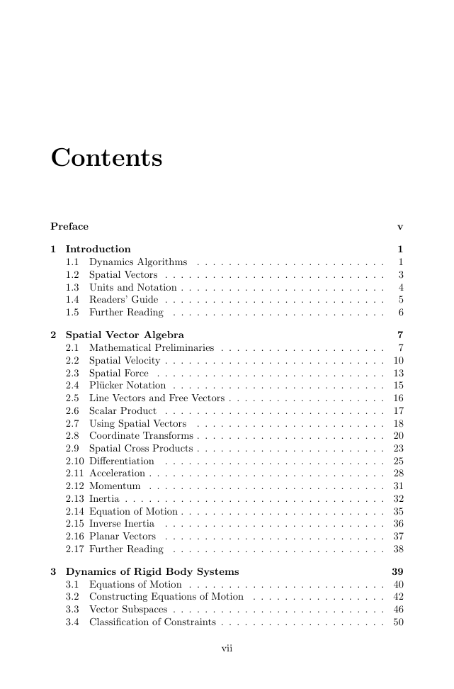
Contents Preface 1 Introduction . . . . . . . . . . . . . . . . . . . . . . . . 1.1 Dynamics Algorithms 1.2 Spatial Vectors . . . . . . . . . . . . . . . . . . . . . . . . . . . . 1.3 Units and Notation . . . . . . . . . . . . . . . . . . . . . . . . . . 1.4 Readers’ Guide . . . . . . . . . . . . . . . . . . . . . . . . . . . . 1.5 Further Reading . . . . . . . . . . . . . . . . . . . . . . . . . . . v 1 1 3 4 5 6 2 Spatial Vector Algebra 7 2.1 Mathematical Preliminaries . . . . . . . . . . . . . . . . . . . . . 7 2.2 Spatial Velocity . . . . . . . . . . . . . . . . . . . . . . . . . . . . 10 2.3 Spatial Force . . . . . . . . . . . . . . . . . . . . . . . . . . . . . 13 2.4 Pl¨ucker Notation . . . . . . . . . . . . . . . . . . . . . . . . . . . 15 2.5 Line Vectors and Free Vectors . . . . . . . . . . . . . . . . . . . . 16 2.6 Scalar Product . . . . . . . . . . . . . . . . . . . . . . . . . . . . 17 2.7 Using Spatial Vectors . . . . . . . . . . . . . . . . . . . . . . . . 18 2.8 Coordinate Transforms . . . . . . . . . . . . . . . . . . . . . . . . 20 2.9 Spatial Cross Products . . . . . . . . . . . . . . . . . . . . . . . . 23 2.10 Diﬀerentiation . . . . . . . . . . . . . . . . . . . . . . . . . . . . 25 2.11 Acceleration . . . . . . . . . . . . . . . . . . . . . . . . . . . . . . 28 2.12 Momentum . . . . . . . . . . . . . . . . . . . . . . . . . . . . . . 31 2.13 Inertia . . . . . . . . . . . . . . . . . . . . . . . . . . . . . . . . . 32 2.14 Equation of Motion . . . . . . . . . . . . . . . . . . . . . . . . . . 35 2.15 Inverse Inertia . . . . . . . . . . . . . . . . . . . . . . . . . . . . 36 2.16 Planar Vectors . . . . . . . . . . . . . . . . . . . . . . . . . . . . 37 2.17 Further Reading . . . . . . . . . . . . . . . . . . . . . . . . . . . 38 3 Dynamics of Rigid Body Systems 39 3.1 Equations of Motion . . . . . . . . . . . . . . . . . . . . . . . . . 40 3.2 Constructing Equations of Motion . . . . . . . . . . . . . . . . . 42 3.3 Vector Subspaces . . . . . . . . . . . . . . . . . . . . . . . . . . . 46 3.4 Classiﬁcation of Constraints . . . . . . . . . . . . . . . . . . . . . 50 vii

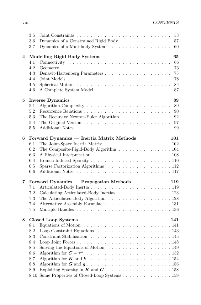
viii CONTENTS 3.5 Joint Constraints . . . . . . . . . . . . . . . . . . . . . . . . . . . 53 3.6 Dynamics of a Constrained Rigid Body . . . . . . . . . . . . . . 57 3.7 Dynamics of a Multibody System . . . . . . . . . . . . . . . . . . 60 4 Modelling Rigid Body Systems 65 4.1 Connectivity . . . . . . . . . . . . . . . . . . . . . . . . . . . . . 66 4.2 Geometry . . . . . . . . . . . . . . . . . . . . . . . . . . . . . . . 73 4.3 Denavit-Hartenberg Parameters . . . . . . . . . . . . . . . . . . . 75 4.4 Joint Models . . . . . . . . . . . . . . . . . . . . . . . . . . . . . 78 4.5 Spherical Motion . . . . . . . . . . . . . . . . . . . . . . . . . . . 84 4.6 A Complete System Model . . . . . . . . . . . . . . . . . . . . . 87 5 Inverse Dynamics 89 5.1 Algorithm Complexity . . . . . . . . . . . . . . . . . . . . . . . . 89 5.2 Recurrence Relations . . . . . . . . . . . . . . . . . . . . . . . . . 90 5.3 The Recursive Newton-Euler Algorithm . . . . . . . . . . . . . . 92 5.4 The Original Version . . . . . . . . . . . . . . . . . . . . . . . . . 97 5.5 Additional Notes . . . . . . . . . . . . . . . . . . . . . . . . . . . 99 6 Forward Dynamics — Inertia Matrix Methods 101 6.1 The Joint-Space Inertia Matrix . . . . . . . . . . . . . . . . . . . 102 6.2 The Composite-Rigid-Body Algorithm . . . . . . . . . . . . . . . 104 6.3 A Physical Interpretation . . . . . . . . . . . . . . . . . . . . . . 108 6.4 Branch-Induced Sparsity . . . . . . . . . . . . . . . . . . . . . . . 110 6.5 Sparse Factorization Algorithms . . . . . . . . . . . . . . . . . . 112 6.6 Additional Notes . . . . . . . . . . . . . . . . . . . . . . . . . . . 117 7 Forward Dynamics — Propagation Methods 119 7.1 Articulated-Body Inertia . . . . . . . . . . . . . . . . . . . . . . . 119 7.2 Calculating Articulated-Body Inertias . . . . . . . . . . . . . . . 123 7.3 The Articulated-Body Algorithm . . . . . . . . . . . . . . . . . . 128 7.4 Alternative Assembly Formulae . . . . . . . . . . . . . . . . . . . 131 7.5 Multiple Handles . . . . . . . . . . . . . . . . . . . . . . . . . . . 136 8 Closed Loop Systems 141 8.1 Equations of Motion . . . . . . . . . . . . . . . . . . . . . . . . . 141 8.2 Loop Constraint Equations . . . . . . . . . . . . . . . . . . . . . 143 8.3 Constraint Stabilization . . . . . . . . . . . . . . . . . . . . . . . 145 8.4 Loop Joint Forces . . . . . . . . . . . . . . . . . . . . . . . . . . . 148 8.5 Solving the Equations of Motion . . . . . . . . . . . . . . . . . . 149 8.6 Algorithm for C − τ a . . . . . . . . . . . . . . . . . . . . . . . . 152 8.7 Algorithm for K and k . . . . . . . . . . . . . . . . . . . . . . . 154 8.8 Algorithm for G and g . . . . . . . . . . . . . . . . . . . . . . . . 156 8.9 Exploiting Sparsity in K and G . . . . . . . . . . . . . . . . . . 158 8.10 Some Properties of Closed-Loop Systems . . . . . . . . . . . . . . 159

资料库

Rigid Body Dynamics Algorithms.pdf

相关推荐

课程资源

热门标签

最新资料