Answers to Selected
Exercises
For
Principles of Econometrics, Fourth Edition
R. CARTER HILL
Louisiana State University
WILLIAM E. GRIFFITHS
University of Melbourne
GUAY C. LIM
University of Melbourne
JOHN WILEY & SONS, INC
New York / Chichester / Weinheim / Brisbane / Singapore / Toronto
�
CONTENTS
Answers for Selected Exercises in:
Probability Primer
Chapter 2
Chapter 3
Chapter 4
Chapter 5
Chapter 6
Chapter 7
Chapter 8
Chapter 9
Chapter 10
Chapter 11
Chapter 15
Chapter 16
Appendix A Mathematical Tools
Appendix B
Appendix C
The Simple Linear Regression Model
Interval Estimation and Hypothesis Testing
Prediction, Goodness of Fit and Modeling Issues
The Multiple Regression Model
Further Inference in the Multiple Regression Model
Using Indicator Variables
Heteroskedasticity
Regression with Time Series Data: Stationary Variables
Random Regressors and Moment Based Estimation
Simultaneous Equations Models
Panel Data Models
Qualitative and Limited Dependent Variable Models
Probability Concepts
Review of Statistical Inference
1
3
12
16
22
29
36
44
51
58
60
64
66
69
72
76
29 August, 2011
�
PROBABILITY PRIMER
Exercise Answers
EXERCISE P.1
(a)
X is a random variable because attendance is not known prior to the outdoor concert.
(b)
(c)
(d)
1100
3500
6,000,000
EXERCISE P.3
0.0478
EXERCISE P.5
(a)
0.5.
(b)
0.25
EXERCISE P.7
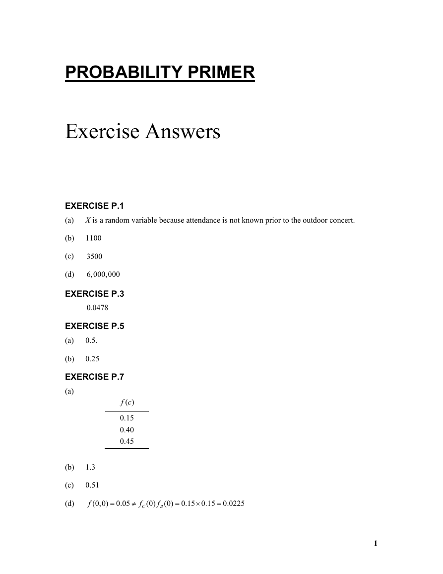
(a)
f c
( )
0.15
0.40
0.45
(b)
(c)
(d)
1.3
0.51
f
(0,0) 0.05
f
C
(0)
f
B
(0) 0.15 0.15 0.0225
1
�
Probability Primer, Exercise Answers, Principles of Econometrics, 4e
2
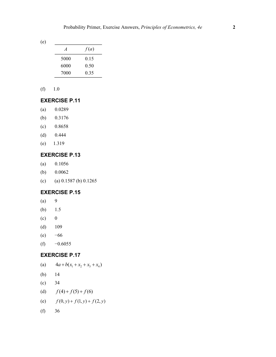
(e)
A
5000
6000
7000
f a
( )
0.15
0.50
0.35
(f)
1.0
EXERCISE P.11
(a)
(b)
(c)
(d)
(e)
0.0289
0.3176
0.8658
0.444
1.319
EXERCISE P.13
(a)
(b)
(c)
0.1056
0.0062
(a) 0.1587 (b) 0.1265
EXERCISE P.15
(a)
(b)
(c)
(d)
(e)
(f)
9
1.5
0
109
−66
−0.6055
EXERCISE P.17
x
(a)
2
(b)
(c)
(d)
(e)
(f)
a b x
4
(
1
14
34
f
(4)
f
(0,
36
(5)
f
(1,
y
)
f
x
3
x
4
)
f
y
)
(6)
f
(2,
y
)
�
CHAPTER 2
Exercise Answers
EXERCISE 2.3
(a)
The line drawn for part (a) will depend on each student’s subjective choice about the
position of the line. For this reason, it has been omitted.
1.514286
b
2
b
1 10.8
(b)
Figure xr2.3 Observations and fitted line
0
1
8
6
4
2
1
2
3
x
4
y
Fitted values
5
6
y
x
ˆ
y
5.5
3.5
5.5
(c)
3
�
Chapter 2, Exercise Answers Principles of Econometrics, 4e
4
Exercise 2.3 (Continued)
(d)
ˆie
0.714286
0.228571
−1.257143
0.257143
−1.228571
1.285714
(e)
ie
ˆ
0.
ix e
ˆ
i
0
240
b
1
is an estimate of the number of sodas sold when the
The intercept estimate
temperature is 0 degrees Fahrenheit. Clearly, it is impossible to sell 240 sodas and so
this estimate should not be accepted as a sensible one.
b is an estimate of the increase in sodas sold when temperature
The slope estimate
2
increases by 1 Fahrenheit degree. One would expect the number of sodas sold to increase
as temperature increases.
ˆ
y
240 8 80
400
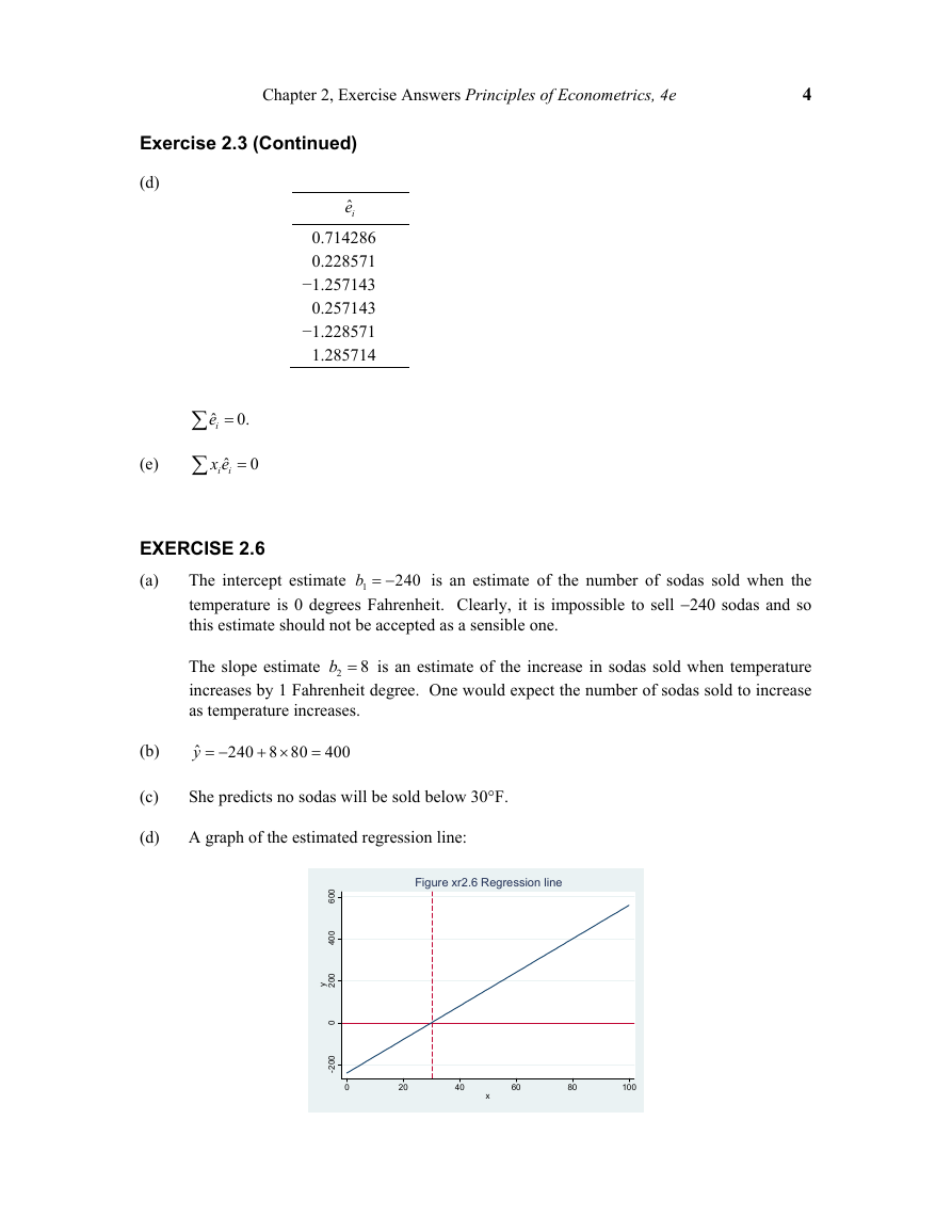
She predicts no sodas will be sold below 30F.
A graph of the estimated regression line:
Figure xr2.6 Regression line
0
0
6
0
0
4
0
0
2
y
0
0
0
2
-
0
20
40
x
60
80
100
EXERCISE 2.6
(a)
8
(b)
(c)
(d)
�
Chapter 2, Exercise Answers Principles of Econometrics, 4e
5
EXERCISE 2.9
(a)
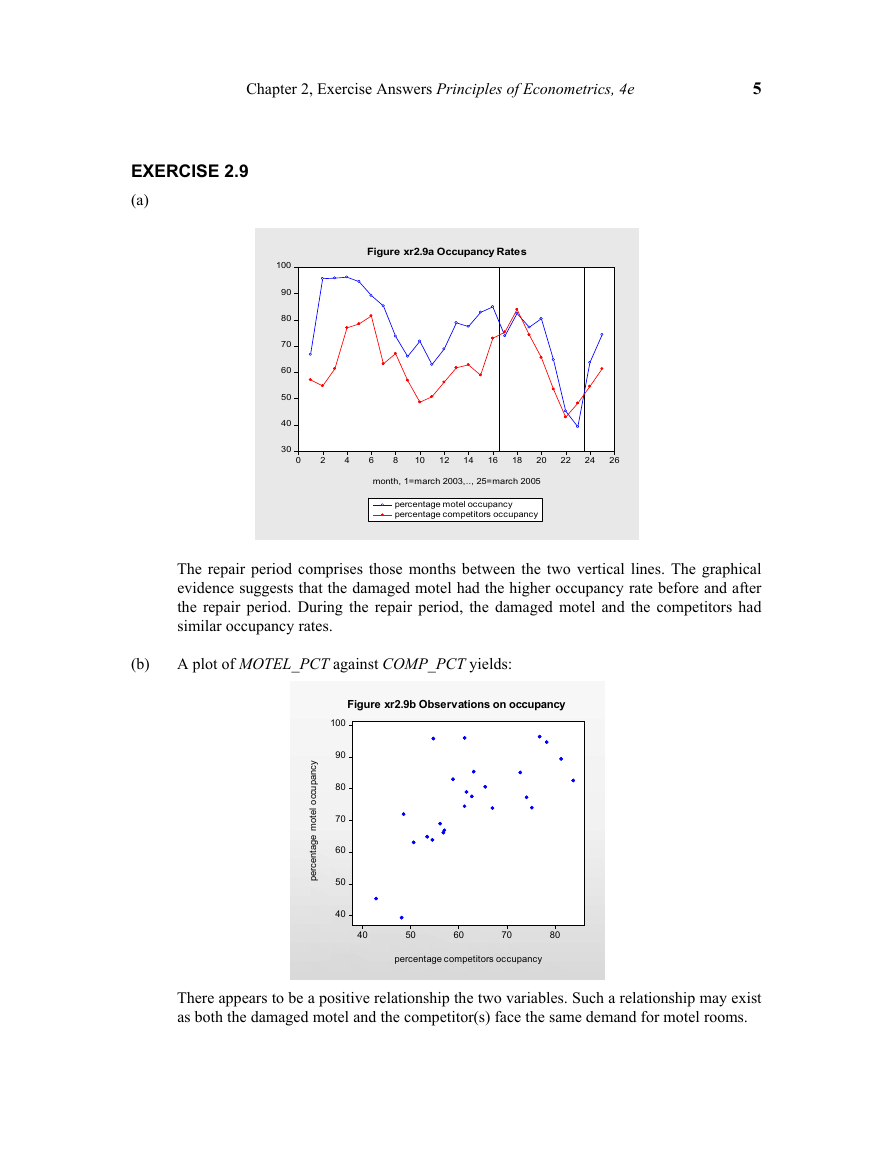
Figure xr2.9a Occupancy Rates
100
90
80
70
60
50
40
30
0
2
4
6
8
10
12
14
16
18
20
22
24
26
month, 1=march 2003,.., 25=march 2005
percentage motel occupancy
percentage competitors occupancy
The repair period comprises those months between the two vertical lines. The graphical
evidence suggests that the damaged motel had the higher occupancy rate before and after
the repair period. During the repair period, the damaged motel and the competitors had
similar occupancy rates.
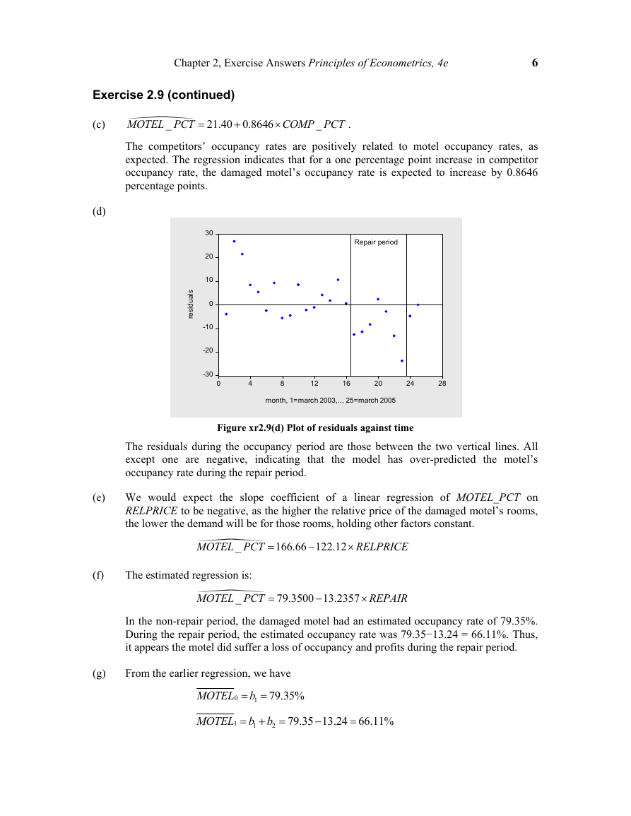
A plot of MOTEL_PCT against COMP_PCT yields:
Figure xr2.9b Observations on occupancy
(b)
100
90
80
70
60
50
40
y
c
n
a
p
u
c
c
o
l
e
t
o
m
e
g
a
t
n
e
c
r
e
p
40
50
60
70
80
percentage competitors occupancy
There appears to be a positive relationship the two variables. Such a relationship may exist
as both the damaged motel and the competitor(s) face the same demand for motel rooms.
�
Chapter 2, Exercise Answers Principles of Econometrics, 4e
6
Exercise 2.9 (continued)
21.40 0.8646
(c) _
MOTEL PCT
The competitors’ occupancy rates are positively related to motel occupancy rates, as
expected. The regression indicates that for a one percentage point increase in competitor
occupancy rate, the damaged motel’s occupancy rate is expected to increase by 0.8646
percentage points.
COMP PCT
_
.
(d)
l
s
a
u
d
s
e
r
i
30
20
10
0
-10
-20
-30
Repair period
0
4
8
12
16
20
24
28
month, 1=march 2003,.., 25=march 2005
Figure xr2.9(d) Plot of residuals against time
The residuals during the occupancy period are those between the two vertical lines. All
except one are negative, indicating that the model has over-predicted the motel’s
occupancy rate during the repair period.
(e) We would expect the slope coefficient of a linear regression of MOTEL_PCT on
RELPRICE to be negative, as the higher the relative price of the damaged motel’s rooms,
the lower the demand will be for those rooms, holding other factors constant.
_
MOTEL PCT
166.66 122.12
RELPRICE
(f)
The estimated regression is:
_
MOTEL PCT
In the non-repair period, the damaged motel had an estimated occupancy rate of 79.35%.
During the repair period, the estimated occupancy rate was 79.35−13.24 = 66.11%. Thus,
it appears the motel did suffer a loss of occupancy and profits during the repair period.
79.3500 13.2357
REPAIR
(g)
From the earlier regression, we have
MOTEL
0
MOTEL
1
b
1 79.35%
b
1
b
2
79.35 13.24 66.11%
�



 2023年江西萍乡中考道德与法治真题及答案.doc
 2012年重庆南川中考生物真题及答案.doc
 2013年江西师范大学地理学综合及文艺理论基础考研真题.doc
 2020年四川甘孜小升初语文真题及答案I卷.doc
 2020年注册岩土工程师专业基础考试真题及答案.doc
 2023-2024学年福建省厦门市九年级上学期数学月考试题及答案.doc
 2021-2022学年辽宁省沈阳市大东区九年级上学期语文期末试题及答案.doc
 2022-2023学年北京东城区初三第一学期物理期末试卷及答案.doc
 2018上半年江西教师资格初中地理学科知识与教学能力真题及答案.doc
 2012年河北国家公务员申论考试真题及答案-省级.doc
 2020-2021学年江苏省扬州市江都区邵樊片九年级上学期数学第一次质量检测试题及答案.doc
 2022下半年黑龙江教师资格证中学综合素质真题及答案.doc