Team#2008495 Page 1 of 19
Problem Chosen
D
2020
MCM/ICM
Summary Sheet
Summary
Soccer Teamwork Evaluation Models
Team Control Number
2008495
This paper proposes a method, with graph theory, probability theory and calculus, to build
machine learning models based on data analysis, which aims at providing strategies for soccer
coach's lineup arrangement and players' training.
Firstly, the Pass Network Model can be established according to the graph theory, whose
edge-weights are evaluation of coordination degree of each dyadic configurations. Pass Evaluate
Index is designed for evaluate a single pass, and the summation of each pass can be defined as
the edge-weights of PNM. For analysis, the adjacency matrix of N participating players within a
period. Several outstanding M configurations can be found by the sort of M-element combination
with the key of the sum of the sub-complete graph edge weights. What’s more, investigation of
the influence of time on pass density depends on the constructed and approximate function of
time and pass.
Secondly, performance indicators that reflect successful teamwork can be divided into
dynamic indicators and static indicators. Static indicators include player position arrangement
and line-up with which player season heatmap models and player position models can be
established while the dynamic indicators include opponents’ strength, side, coach, passes,
defense, attack and fail. etc. After visualized analysis of the correlation between the dynamic
indicators extracted after data cleaning, and with the setting label by the goal difference, the
random forest classifier, a machine learning model, is used as a evaluation model of dynamic
indicators. After the Grid Search used for tuning parameters, and cross-validation, the accuracy
of the model achieving 80% approximately.
Thirdly, the study focuses on the role of static indicators in the performance of the team and
in different positions which
establishes different players' value evaluation models
comprehensively consider the player’s positions and technical statistical data evaluation. To
optimize the value of 11-person permutation, we choose simulated annealing (SA) algorithm
which searches the global optimal solution in cousin points in the same minimized search tree
after the local optimal solution has attained. The model finally gave the best starting lineup
formation. In addition, we also consider the following three secondary factors: tacit
understanding between players, home and away influence, and coaching arrangements. All
analysis above can be concluded as comprehensive suggestion to the coach.
Finally, we use the case of the Huskies to explain group dynamics. And use the conclusions
obtained by the Huskies to build a model to explain how to design a more effective team and
supplement the team performance indicators.
Key words: Network; Graph theory; Calculus; Machine learning; Random forest classifier;
Simulated annealing; Heat map; Group dynamics
�
Team#2008495 Page 2 of 19
5
1
2
Introduction.................................................................................................................................................. 3
1.1 Background ......................................................................................................................................................... 3
1.2 Problem Restatement .......................................................................................................................................... 3
Preparation of the Models ............................................................................................................................ 3
2.1 Processing Tools .................................................................................................................................................. 3
2.2 Data Cleaning ...................................................................................................................................................... 4
Establishment of PNM and Analysis of Influence Factors .............................................................................. 4
3.1 Pass Evaluation Index(PEI) ............................................................................................................................. 4
3.2 Pass Network Model (PNM) and Recognition of Network Pattern ..................................................................... 6
3.3 Fluctuation of Passing State at The Time ............................................................................................................ 6
Soccer Team Indexes and Performance Prediction Based on ML ................................................................... 7
4.1 Static Index (SI) .................................................................................................................................................... 8
4.2 Dynamic Index (DI) .............................................................................................................................................. 9
4.2.1 Data Cleaning and Feature Engineering ...................................................................................................... 9
4.2.2 Visualization Analysis .................................................................................................................................. 9
4.2.3 RFC Establishment, Optimization, and Training......................................................................................... 12
Design of Structural Strategies Driven by SA ............................................................................................... 13
5.1 Position Evaluation Engineering (PEE) .............................................................................................................. 13
5.2 Optimization of Permutation and Combination Based on SA Algorithm .......................................................... 14
5.3 Other Structural Strategy Factors ..................................................................................................................... 15
5.4 Structural Strategy Conclusion .......................................................................................................................... 16
6 Model Extension Combined with Group Dynamics ..................................................................................... 16
6.1 Group and Soccer Team .................................................................................................................................... 17
6.1.1 Group Cohesiveness .................................................................................................................................. 17
6.1.2 Group Standard and Group Pressure ........................................................................................................ 17
6.1.3 Individual Motivation and Group Goals .................................................................................................... 17
6.1.4 Leadership and Group Performance ......................................................................................................... 18
6.1.5 Group Structure ........................................................................................................................................ 18
6.2 Other influence factor of successful teamwork ................................................................................................. 18
Evaluation ................................................................................................................................................... 18
7.1 Strength ............................................................................................................................................................ 18
7.2 Weakness....................................................................................................................................................... 19
Reference ................................................................................................................................................... 19
3
4
7
8
2
�
Team#2008495 Page 3 of 19
1 Introduction
Football has a long history. It has been loved all over the world since it was popularized.
Football can be considered as the most popular sports in the world. Football, a seemingly simple
sport, contains the secrets of individual ability and team cooperation. With the development of
the times and the progress of science and technology, football players and coaches continue to
improve in skills, showing the audience wonderful matches. As we all know, a wonderful
football match is inseparable from the contributions of players and teams. By studying the
actions of everyone in the team, coordinating the team relationship, reasonably arranging the
minutes and line-up, we can score best.
Football is a sport suitable for all ages. Since its inclusion in international tournaments,
people have created a variety of methods to evaluate the team dynamics throughout the match
and over the entire season to help determine specific strategies that can improve teamwork next
season. We need to use the data provided by the ICM team to build a model to solve the
following four problems.
1. Consider each player as a node and create a passing network to identify dyadic, triadic and
multiple configurations. We need to establish a value evaluation model of a single pass and a
general evaluation model of the passing of the time structure index under the passing
network.
2. To Identify performance indicators that reflect successful teamwork, we need to consider
static and dynamic indicators. Establish a model of the impact of each performance indicator
on successful teamwork, and use one model to encompass these four sub-models.
3. By observing and analyzing the model established in Questions 1 and 2, tell the coach that
which form of structural strategy is applicable to the Huskies. Using the results of the model
analysis to make suggestions for the coach to improve the team's success rate next season.
4. Use the case of the Huskies to explain the theory of group dynamics, and use the conclusion
of the model established by the Huskies to explain how to design a more effective team, and
supplement the team performance indicators.
2 Preparation of the Models
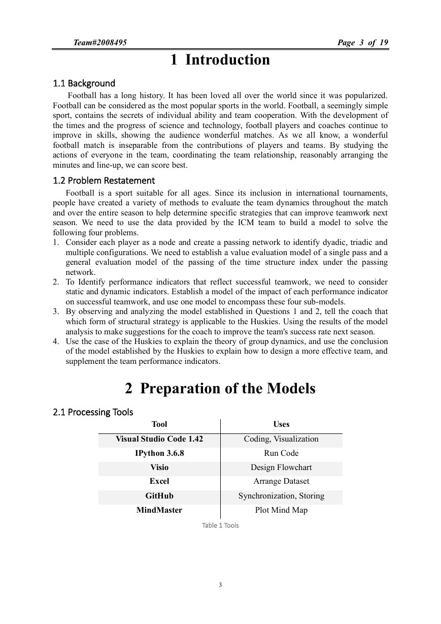
Tool
Uses
Visual Studio Code 1.42
Coding, Visualization
IPython 3.6.8
Visio
Excel
GitHub
MindMaster
Run Code
Design Flowchart
Arrange Dataset
Synchronization, Storing
Plot Mind Map
3
�
Team#2008495 Page 4 of 19
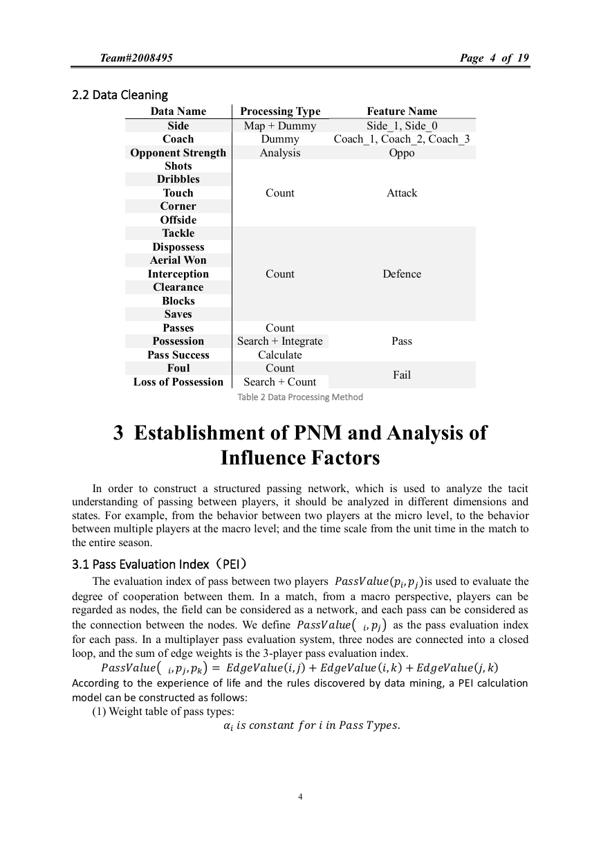
Processing Type
Map + Dummy
Dummy
Analysis
Feature Name
Side_1, Side_0
Coach_1, Coach_2, Coach_3
Oppo
Count
Attack
Count
Defence
Data Name
Side
Coach
Opponent Strength
Shots
Dribbles
Touch
Corner
Offside
Tackle
Dispossess
Aerial Won
Interception
Clearance
Blocks
Saves
Passes
Possession
Pass Success
Foul
Count
Search + Integrate
Calculate
Count
Pass
Fail
Loss of Possession
Search + Count
3 Establishment of PNM and Analysis of
Influence Factors
In order to construct a structured passing network, which is used to analyze the tacit
understanding of passing between players, it should be analyzed in different dimensions and
states. For example, from the behavior between two players at the micro level, to the behavior
between multiple players at the macro level; and the time scale from the unit time in the match to
the entire season.
for each pass. In a multiplayer pass evaluation system, three nodes are connected into a closed
loop, and the sum of edge weights is the 3-player pass evaluation index.
degree of cooperation between them. In a match, from a macro perspective, players can be
regarded as nodes, the field can be considered as a network, and each pass can be considered as
The evaluation index of pass between two players (,)is used to evaluate the
the connection between the nodes. We define , as the pass evaluation index
,,= (,)+(,)+(,)
(1) Weight table of pass types: .
According to the experience of life and the rules discovered by data mining, a PEI calculation
model can be constructed as follows:
4
�
Team#2008495 Page 5 of 19
(2) Calculate pressure from defenders when passing or receiving
weighted average of the pressure from defenders, quantified as the following formula:
For x is the abscissa from the player to the opponent's gate, and it is negatively related to the
pressure from defenders.
()=1−12tan[116×(100−0.6)]
(,)= ,
(3)Single pass evaluation, (,), is the weight of the pass type multiplied by
,= ∗ ∗0.3+()∗0.7
According to this pass evaluation index model, an adjacency matrix of all N players
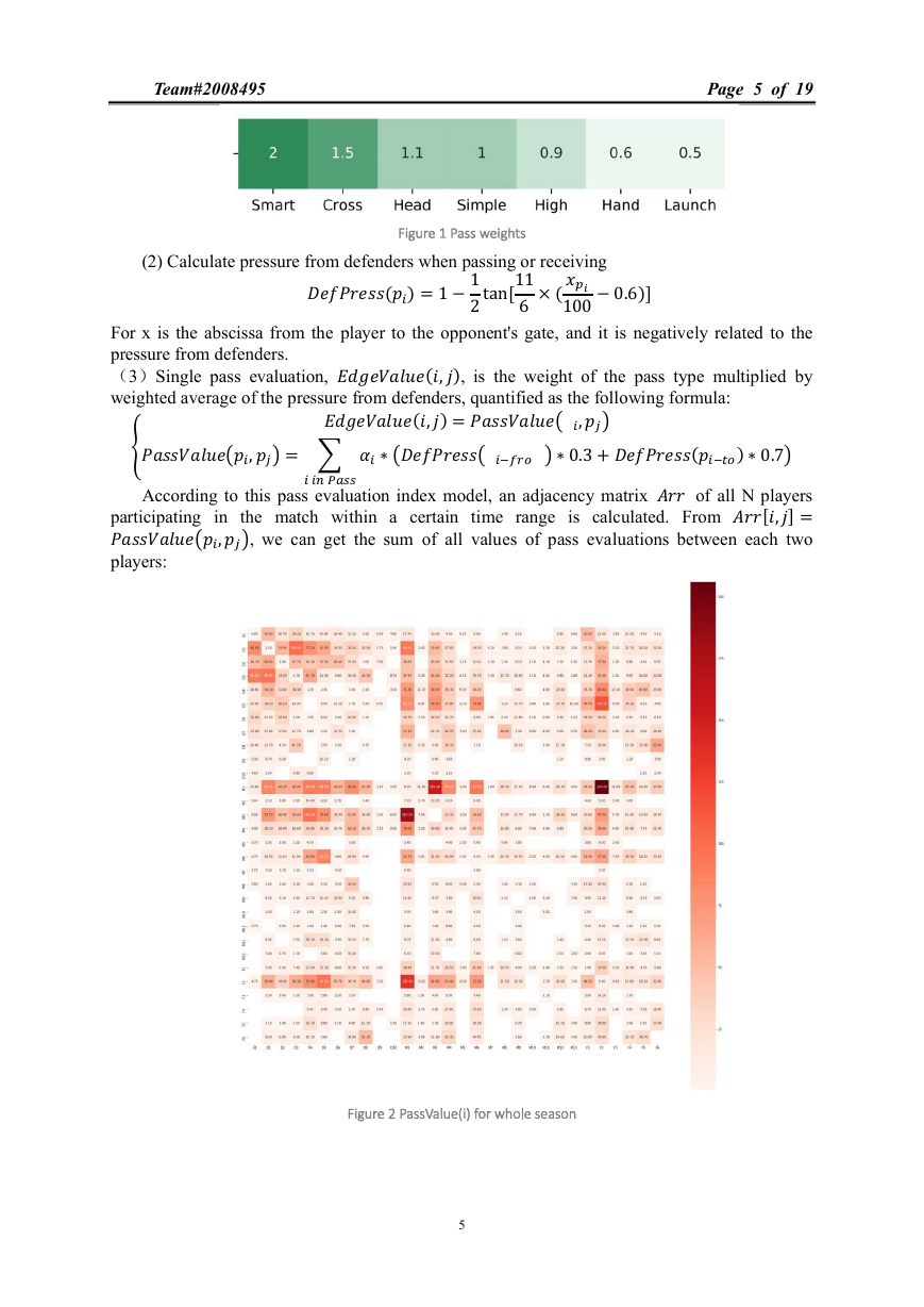
participating in the match within a certain time range is calculated. From [,]=
,, we can get the sum of all values of pass evaluations between each two
players:
5
�
Team#2008495 Page 6 of 19
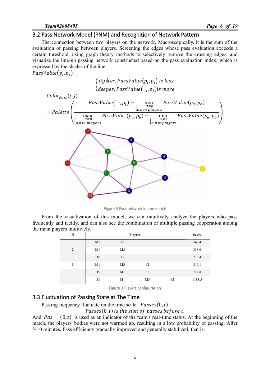
The connection between two players on the network, Macroscopically, it is the sum of the
evaluation of passing between players. Screening the edges whose pass evaluation exceeds a
certain threshold, using graph theory methods to selectively remove the crossing edges, and
visualize the line-up passing network constructed based on the pass evaluation index, which is
expressed by the shades of the line.
,:
ℎ,,
, ,
(,)
, (,)
min
,−
, (,)
=
, (,)−
min
max
From the visualization of this model, we can intuitively analyze the players who pass
frequently and tacitly, and can also see the combination of multiple passing cooperation among
the main players intuitively.
N
2
3
4
M1
M1
D5
M1
D5
D5
Players
F2
F2
M3
F2
M3
F2
M3
M1
M1
Score
342.4
338.6
213.4
816.1
727.8
F2
1113.5
Passing frequency fluctuate on the time scale. (0,)
And
(0,) is used as an indicator of the team's real-time status. At the beginning of the
(0,) ℎ .
match, the players' bodies were not warmed up, resulting in a low probability of passing. After
5-10 minutes, Pass efficiency gradually improved and generally stabilized, that is:
6
�
{ (0,)>0
(0,)<0
lim→(0,)=
<
2
(0,)<0
{
(0,)>0
lim→(0,)=<
>
2
(,)= ()
As the time goes, the players' physical strength and the pass density decrease, that is, the
increase in the number of passes slows down (although the number of successful passes in a
match is still increasing, the frequency of pass failure begins to increase), after that the pass
density Showing a downward trend, that is:
Looking at the pass frequency density of players in 38 matches throughout the season, the
whole the trend of frequency density is similar to that shows in a single match. Plot with time as
the abscissa and successful pass density as the ordinate:
Team#2008495 Page 7 of 19
Generally, the density of passes is relatively stable in a time scale. If we use the Monte Carlo
method to simulate each pass, the time probability distribution for the next pass after the last pass
is set to obey (0,1), where is the statistical average of interval time of pass. Then when the
sample size N satisfies log≈2, it will approximate the distribution on the left graph; as the
sample size increases, when log>4 is satisfied, it will approximate the distribution on the
obeys (0,1).
right graph. Therefore, we can consider that the probability of passing events at each time point
4 Soccer Team Indexes and Performance
Prediction Based on ML
There are many indicators for successful teamwork in a football team. Based on data
analysis and practical experience, we mainly consider the following indicators: static indicators
and dynamic indicators. First, we use () to evaluate the overall performance of a team in
a match. define ():
−<−1
−∈[−1,1]
−>1
()=−1,
0,
1,
7
�
Team#2008495 Page 8 of 19
In order to consider the distribution of players’ positions, we took the position coordinates of
each player throughout the season and made a heat map. The value of each point in the heat map
is defined as follows:
[,]= 14 1, ℎ ℎ
0,
,>0
[,], the position heat map of the main 11 players is got as follows:
The darker the color is, the more active the player is in this position. After calculating
In a match, team formation plays an important role in collaboration. We want to find out
what the formation is like. We take the coordinates of each player in each match and integrate the
coordinates over time to find out the average coordinates. We take the time which can be got
from data (Origin / Destination Player) as the new abscissa, and the X or Y coordinate as the new
ordinate, so we got functions X (t) and Y (t). Approximately, we thought that between any two
closest recorded time points, the player moves at a constant speed in the X or Y direction, so that
the discrete data set is converted into a continuous dataset for each match. The average
coordinate, taking the X coordinate as an example (the Y coordinate is the same), is:
() , ℎ ℎ .
≈12(−)×
()=
()
=
Plot these 11 players’ average coordinate on the map, we got the formation graph of each
match. Some of them are as follows:
8
�



 2023年江西萍乡中考道德与法治真题及答案.doc
 2012年重庆南川中考生物真题及答案.doc
 2013年江西师范大学地理学综合及文艺理论基础考研真题.doc
 2020年四川甘孜小升初语文真题及答案I卷.doc
 2020年注册岩土工程师专业基础考试真题及答案.doc
 2023-2024学年福建省厦门市九年级上学期数学月考试题及答案.doc
 2021-2022学年辽宁省沈阳市大东区九年级上学期语文期末试题及答案.doc
 2022-2023学年北京东城区初三第一学期物理期末试卷及答案.doc
 2018上半年江西教师资格初中地理学科知识与教学能力真题及答案.doc
 2012年河北国家公务员申论考试真题及答案-省级.doc
 2020-2021学年江苏省扬州市江都区邵樊片九年级上学期数学第一次质量检测试题及答案.doc
 2022下半年黑龙江教师资格证中学综合素质真题及答案.doc