Convolutional Deep Belief Networks on CIFAR-10
Alex Krizhevsky
kriz@cs.toronto.edu
1
Introduction
We describe how to train a two-layer convolutional Deep Belief Network (DBN) on the 1.6 million tiny images
dataset.
When training a convolutional DBN, one must decide what to do with the edge pixels of teh images. As
the pixels near the edge of an image contribute to the fewest convolutional �lter outputs, the model may
see it �t to tailor its few convolutional �lters to better model the edge pixels. This is undesirable becaue it
usually comes at the expense of a good model for the interior parts of the image. We investigate several ways
of dealing with the edge pixels when training a convolutional DBN. Using a combination of locally-connected
convolutional units and globally-connected units, as well as a few tricks to reduce the e�ects of over�tting,
we achieve state-of-the-art performance in the classi�cation task of the CIFAR-10 subset of the tiny images
dataset.
2 The dataset
Throughout this paper we employ two subsets of the 80 million tiny images dataset [2]. The 80 million
tiny images dataset is a collection of 32 × 32 color images obtained by searching various online image search
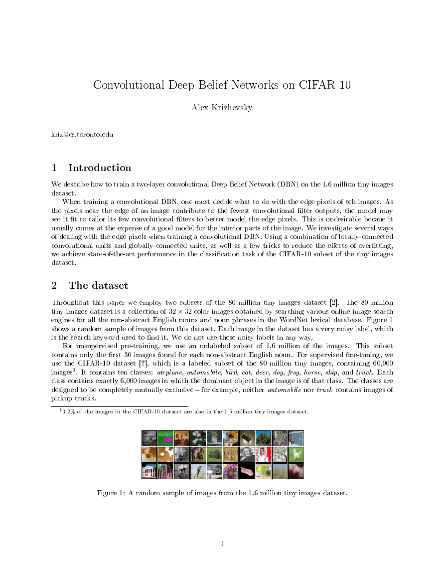
engines for all the non-abstract English nouns and noun phrases in the WordNet lexical database. Figure 1
shows a random sample of images from this dataset. Each image in the dataset has a very noisy label, which
is the search keyword used to �nd it. We do not use these noisy labels in any way.
For unsupervised pre-training, we use an unlabeled subset of 1.6 million of the images. This subset
contains only the �rst 30 images found for each non-abstract English noun. For supervised �ne-tuning, we
use the CIFAR-10 dataset [?], which is a labeled subset of the 80 million tiny images, containing 60,000
images1. It contains ten classes: airplane, automobile, bird, cat, deer, dog, frog, horse, ship, and truck. Each
class contains exactly 6,000 images in which the dominant object in the image is of that class. The classes are
designed to be completely mutually exclusive � for example, neither automobile nor truck contains images of
pickup trucks.
13.2% of the images in the CIFAR-10 dataset are also in the 1.6 million tiny images dataset.
Figure 1: A random sample of images from the 1.6 million tiny images dataset.
1
�
3 Past work
Convolutional models and DBNs have been in use for years.
In [5], the authors trained a convolutional
DBN to recognize digits from the MNIST dataset. More directly related to this work, [1] trained a fully-
connected two-layer DBN on the tiny images dataset and �ne-tuned the model's features with a logistic
regression classi�er. The author achieved a 65% accuracy on the CIFAR-10 test set. In [7], the authors train
a �mcRBM� to achieve a 71.0% accuracy rate. In [6], the authors achieve 74.5% with a sparse-coding scheme.
This is currently the best-published result.
4 Models
4.1 Overview of our methods
Brie�y speaking, we train a convolutional DBN on the 1.6 million tiny images dataset, and then use it to
initialize a convolutional neural net. We then �ne-tune the weights of the convolutional net to classify images
from the CIFAR-10 dataset using a logistic regression classi�er at the output of the net. [4] is an excellent
reference for training Restricted Boltzmann Machines (RBMs) in general.
To learn features from unlabeled color images in an unsupervised manner, we build upon the work of [1],
in which the author trained a two-layer Gaussian-Bernoulli DBN on color images. However, the DBN in that
work was fully connected to the image pixels, while we instead focus on convolutional models. In addition,
we adopt the use of �ReLU�s (REcti�ed Linear Units) in the hidden layer, following [8]. Our tests con�rm
that these units are in fact superior to Bernoulli units. Given input x, the output of a ReLU unit is
y = max(x, 0).
Our ReLU units di�er from those of [8] in two respects. First, we cap the units at 6, so our ReLU activation
function is
y = min(max(x, 0), 6).
In our tests, this encourages the model to learn sparse features earlier.
In the formulation of [8], this is
equivalent to imagining that each ReLU unit consists of only 6 replicated bias-shifted Bernoulli units, rather
than an in�nute amount. We will refer to ReLU units capped at n as ReLU-n units.
Additionally, we employ a di�erent noise model than that of [8].
[8] computes that in order to sample
from a ReLU unit, one must add Gaussian noise with standard deviation
to the unit's mean-�eld activity y. We instead add noise with standard deviation
1
1 + e−x
0 : if y = 0 or y = 6
1 : if 0 < y < 6
.
For values of y approaching 6, the two noise models are identical. But for values of y slightly greater than
zero, our model adds signi�cantly more noise. We believe this encourages the model to learn features that
are almost always o�, as features that are frequently on will incur a high variance (noise) penalty. Both of
these modi�cations to ReLU units are similar in spirit to the various sparseness-inducing tricks commonly
employed when training unsupervised models on natural images. They also happen to be extremely cheap
computationally.
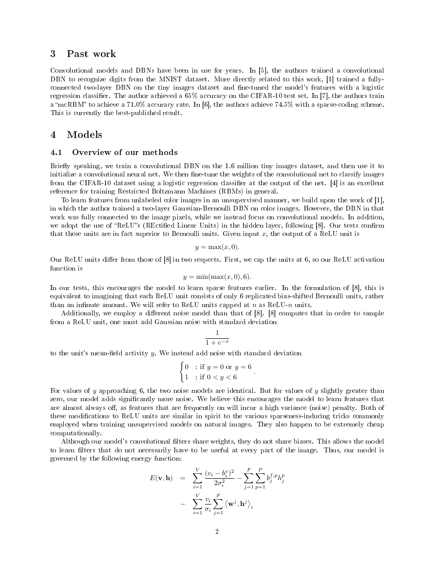
Although our model's convolutional �lters share weights, they do not share biases. This allows the model
to learn �lters that do not necessarily have to be useful at every part of the image. Thus, our model is
governed by the following energy function:
E(v, h) =
P
p=1
− F
wj, hj
j=1
i
j hp
bf,p
j
V
− V
i=1
i=1
(vi − bv
i )2
2σ2
i
vi
σi
F
j=1
2
�
produced when wj is convolved with the image, andwj, hj
where v, h are the visible and hidden unit activities, respectively, V is the number of visible units, F is the
number of convolutional �lters, bv
i is the ith visible bias, σi is the standard deviation of the ith visible unit, P
is the number of outputs that a �tler produces when convolved with an image, bf,p
is the bias of the jth �lter
at position p, hp
j is the activity of the jth �lter at position p, wj is the jth �lter, hj is the grid of activities
i is the ith output when hj is convolved with
wj rotated by 180 degrees.
We use convolutional �lters of size 9× 9, for several reasons. First, 9× 9 is big enough to capture the scale
of most edges and other salient features in the image. Second, 9 × 9 �lters lead to a convolutional output
grid of dimensions 24 × 24, which can be easily divided into subsquares of 3 × 3, 4 × 4, or 6 × 6, making local
pooling simple. Third, odd-sized �lters can lead to nicely centered features.
j
One of the �rst di�culties in training a convolutional RBM is dealing with the boundary pixels. Since
these pixels contribute to far fewer hidden unit activities than do interior pixels, the convolutional RBM
tends to have di�culty modeling them. Typically, the RBM gets around this by learning �lters that are
zero everywhere except near one of the four corners. That is, it will attempt to make every �lter useful for
modeling the boundaries (and especially the corners) of the image, and it will do so by learning corner �lters.
Since we do not wish our model to focus overtly on the boundaries and corners of images � the interior of
the image is much more likely to contain useful hints about the class label � we investigate several methods
for dealing (or not dealing) with this boundary problem. These are
1. Not dealing with the boundary in any special way.
2. Adding a border of zeros around the image. We use a padding of width 4 in order to encourage the
RBM to learn centered �lters and not to focus overtly on the boundary.
3. Using some number of globally-connected units in addition to the convolutional units.
Ideally, the
global units should learn to focus on the boundaries of the image, freeing the convolutional units from
that task.
4. Combining 2 and 3.
5. Holding �xed the pixels of the image that are near the boundary � perhaps those that are half a �lter-
width away. This is, in a sense, of the converse of adding a border of zeros around the image. It is less
computationally expensive than adding a border of zeros, and should also instruct the RBM to learn
centered �lters and not to focus overtly on the boundary, since the RBM will never have to reconstruct
it.
6. Combining 3 and 5.
After training the convolutional RBM, we use it to generate features from images by computing the hidden
unit activations for each image. In the case when we do not add any zero padding to the images, each �lter
produces a 24 × 24 output grid when applied to an image. We subsample this grid using 4 × 4 overlapping
local-max regions, as illustrated in Figure 2. This reduces the feature dimensionality from f×24×24 = f×576
to f × 24 × 24/16 + f × 20 × 20/16 = f × 61, where f is the number of convolutional �lters. The case with
zero padding is analogous, except that the output grid that we subsample is 32 × 32 rather than 24 × 24.
After subsampling, we obtain a feature vector with values in the range [0, 6] (the range of the ReLU-6
unit activations). We wish to use the weights from the convolutional RBM to initialize a convolutional neural
net, which will be trained to classify the images in the CIFAR-10 dataset. It turns out that when placed at
the lower levels of the net, units with such a large linear range (0-6) encourage the net to simply memorize
the training data rather than generalize to new examples. So we cap the ReLU activations at 1, to obtain
a feature vector with values in the range [0, 1]. Fortunately, the features that the convolutional RBM learns
are very sparse. Few of them ever have activations greater than 1. So we do not lose much resolution by
capping the ReLU activations. Figure 3 shows a histogram of ReLU feature activations on a random subset
of 100 images (after the cap at 1).
We train an ordinary, fully-connected RBM on these convolutional ReLU-1 features. This RBM has
ReLU-1 visible units and ReLU-6 hidden units (the number of hidden units in this RBM is either the same
or almost the same as the number of visibles). We opt not to train a convolutional RBM in the second layer
because the �images� on which it would be trained are only 6 × 6 pixels.
3
�
Figure 2: The local-pooling grid that we use. Each pictured 4 × 4 square is subsampled (using max) to one
value.
Figure 3: Histogram of mean-�eld ReLU feature activations on a random subset of 100 images, after capping
the activations at 1. Notice how sparse the features are and how rare activations greater than 1 must have
been prior to capping. 90% of the activations are in the range [0, 0.1), and 79% of the activations are exactly
zero.
4
�
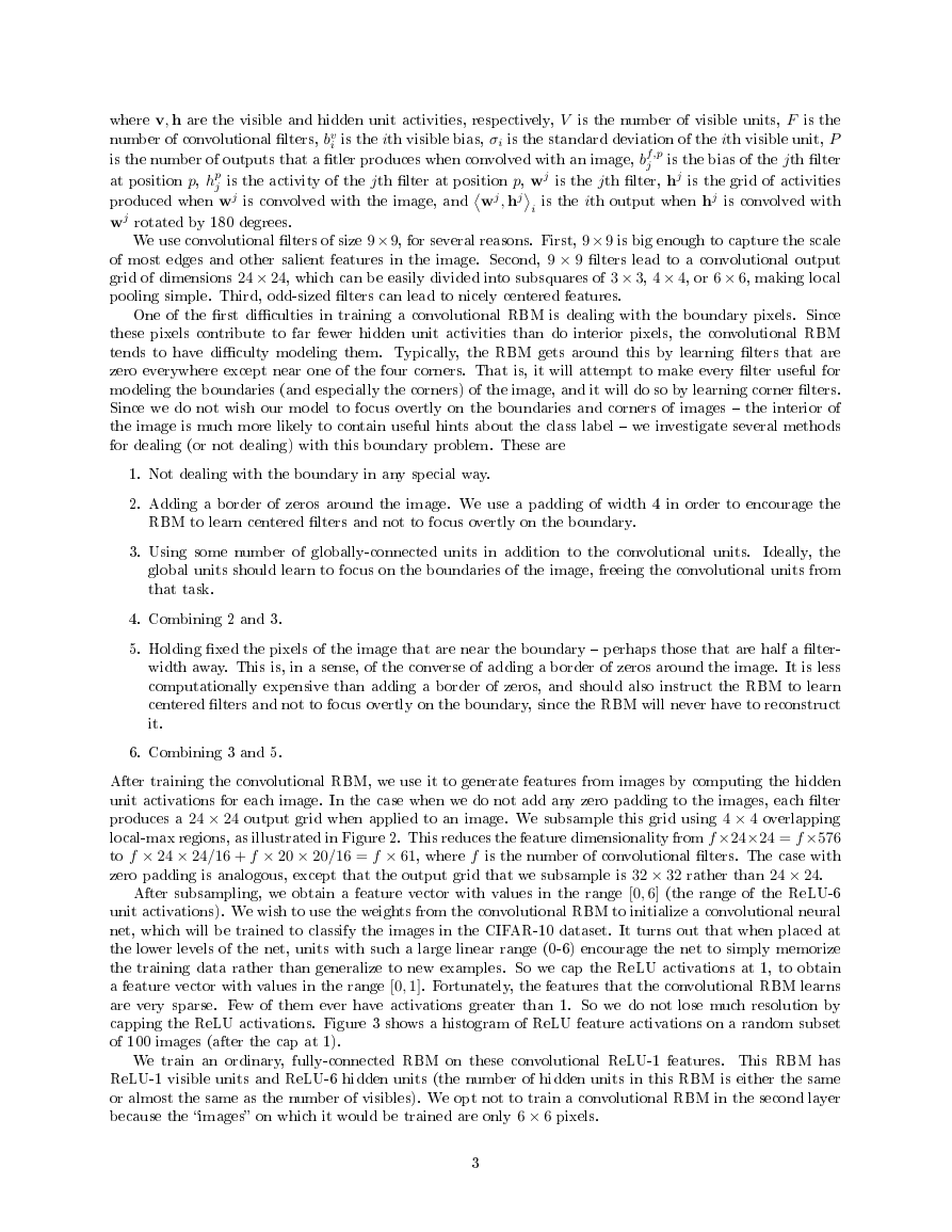
Figure 4: The architecture of our convolutional net. The case with globally-connected units is shown here.
The overlapping max-pooling operation is as illustrated in Figure 2. The classi�er at the output of the net
is multinomial logistic regression.
After training the second-layer RBM, we initialize a two-layer convolutional net with the weights from
the two RBMs and �ne-tune it to classify the images in the CIFAR-10 dataset, using multinomial logistic
regression at the output. Figure 4 illustrates the architecture of the net in the case when we also have
globally-connected units.
The most computationally-intensive networks that we describe here take 45 hours to pre-train and 36
hours to �ne-tune on an Nvidia GTX 280 GPU. By far, most of the time is spent squeezing the last few
fractions of a percent from the nets.
4.2 Details of learning
4.2.1 Dataset
We pre-process the 1.6 million tiny images dataset by deleting the 1000 least-signi�cant principal components.
The pre-processed images look identical to the original images to the naked eye. We also subtract the mean
and set the average standard deviation over all dimensions to 1.
4.2.2 Pre-training
We initialize all weights in both layers from a normal distribution with mean zero and standard deviation
10−3, and we initialize all biases at zero. We train both RBMs using CD-1 [3]; the �rst for 45 epochs2 and
the second for 30. We do not add any noise when reconstructing the pixels from the hidden activities in
either RBM. We use a mini-batch size of 1283. We also use a momentum of 0.9 on the weights and biases for
both RBMs. Thus, the weight update for mini-batch i is the learning rate4 times the average gradient for
mini-batch i plus 0.9 times the previous weight update.
For the �rst-layer convolutional RBM, we use a learning rate of 5 · 10−6 on the visible-convolutional
weights, 5 · 10−5 on the visible and hidden unit biases, 10−3 on the visible-global weights (if any), and 10−2
2An epoch is one cycle through the training data.
3128 happens to be a good number to use on Nvidia GPUs because it leads to matrices whose dimensions are divisible by
64. Multiplication of such matrices is about 50% faster.
4The learning rate is the multiplier of the average gradient for a mini-batch of images.
5
�
Parameter
Visible-convolutional weights
Visible-global weights
Second-layer weights
Output weights
Convolutional unit biases
Global unit biases
Second-layer unit biases
Output unit biases
10−4
2.5 · 10−6
2 · 10−4
10−3
10−4
2 · 10−4
2 · 10−4
10−3
Learning rate Momentum Weight decay coe�cient
0.9
0
0.9
0.9
0.9
0.9
0.9
0.9
0
0
0
8 · 10−3
0
0
0
0
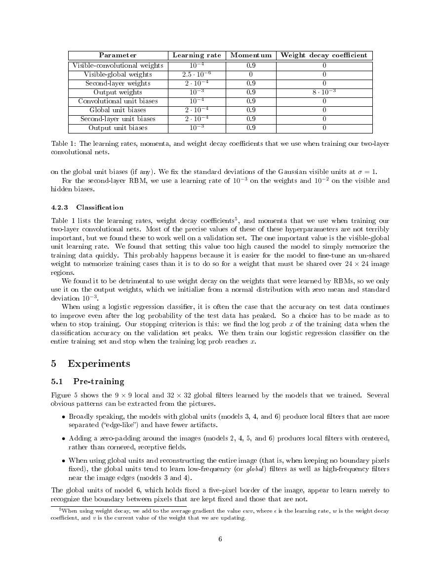
Table 1: The learning rates, momenta, and weight decay coe�cients that we use when training our two-layer
convolutional nets.
on the global unit biases (if any). We �x the standard deviations of the Gaussian visible units at σ = 1.
For the second-layer RBM, we use a learning rate of 10−3 on the weights and 10−2 on the visible and
hidden biases.
4.2.3 Classi�cation
Table 1 lists the learning rates, weight decay coe�cients5, and momenta that we use when training our
two-layer convolutional nets. Most of the precise values of these of these hyperparameters are not terribly
important, but we found these to work well on a validation set. The one important value is the visible-global
unit learning rate. We found that setting this value too high caused the model to simply memorize the
training data quickly. This probably happens because it is easier for the model to �ne-tune an un-shared
weight to memorize training cases than it is to do so for a weight that must be shared over 24 × 24 image
regions.
We found it to be detrimental to use weight decay on the weights that were learned by RBMs, so we only
use it on the output weights, which we initialize from a normal distribution with zero mean and standard
deviation 10−3.
When using a logistic regression classi�er, it is often the case that the accuracy on test data continues
to improve even after the log probability of the test data has peaked. So a choice has to be made as to
when to stop training. Our stopping criterion is this: we �nd the log prob x of the training data when the
classi�cation accuracy on the validation set peaks. We then train our logistic regression classi�er on the
entire training set and stop when the training log prob reaches x.
5 Experiments
5.1 Pre-training
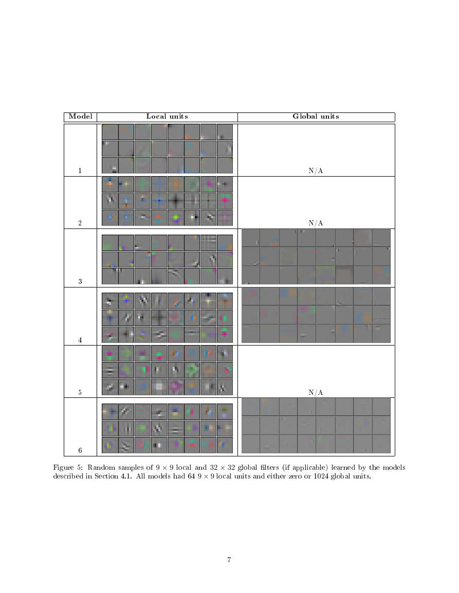
Figure 5 shows the 9 × 9 local and 32 × 32 global �lters learned by the models that we trained. Several
obvious patterns can be extracted from the pictures.
• Broadly speaking, the models with global units (models 3, 4, and 6) produce local �lters that are more
separated (�edge-like�) and have fewer artifacts.
• Adding a zero-padding around the images (models 2, 4, 5, and 6) produces local �lters with centered,
rather than cornered, receptive �elds.
• When using global units and reconstructing the entire image (that is, when keeping no boundary pixels
�xed), the global units tend to learn low-frequency (or global ) �lters as well as high-frequency �lters
near the image edges (models 3 and 4).
The global units of model 6, which holds �xed a �ve-pixel border of the image, appear to learn merely to
recognize the boundary between pixels that are kept �xed and those that are not.
5When using weight decay, we add to the average gradient the value �wv, where � is the learning rate, w is the weight decay
coe�cient, and v is the current value of the weight that we are updating.
6
�
Model
Local units
Global units
1
2
3
4
5
6
N/A
N/A
N/A
Figure 5: Random samples of 9 × 9 local and 32 × 32 global �lters (if applicable) learned by the models
described in Section 4.1. All models had 64 9 × 9 local units and either zero or 1024 global units.
7
�
Model Two-layer performance
(a)
3
4
5
6
77.46%
78.90%
77.56%
77.27%
Number of layers Model 4 performance
(b)
1
1 + pooling
2
70.67%
75.12%
78.90%
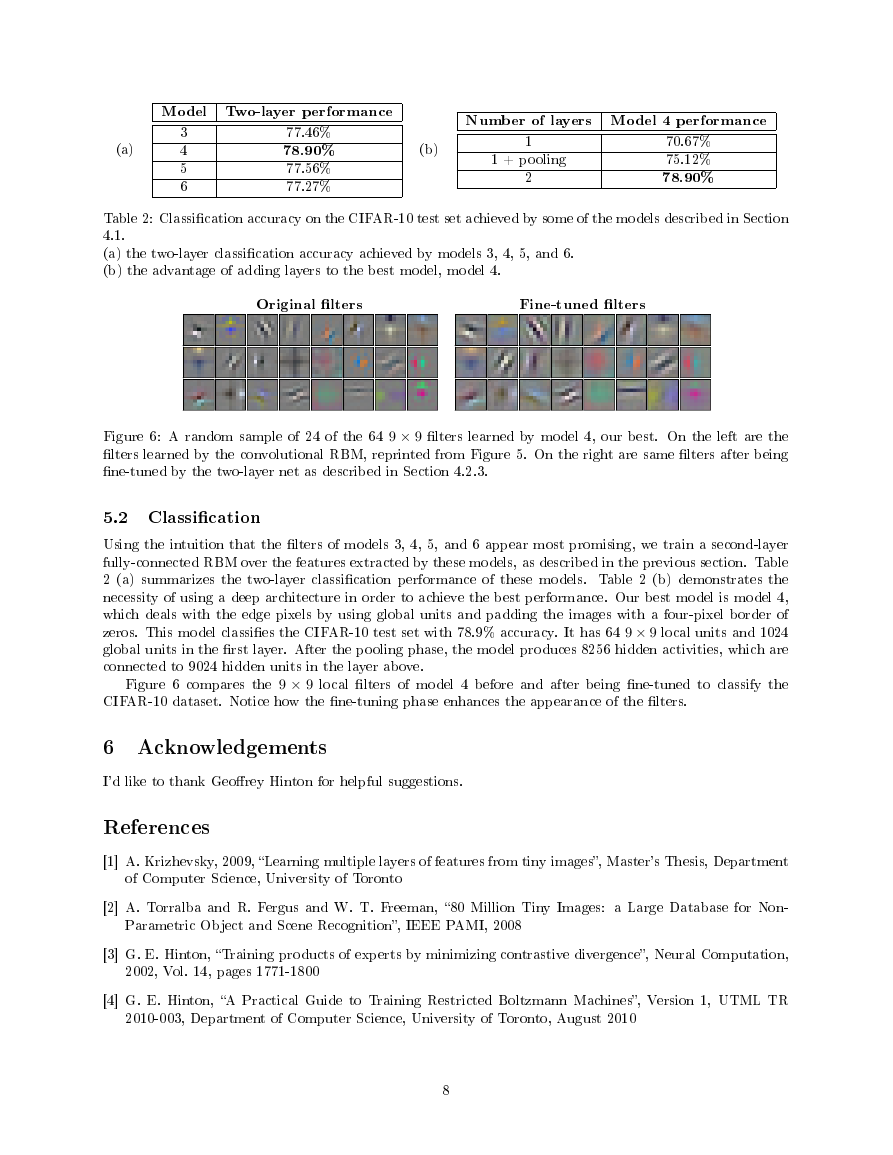
Table 2: Classi�cation accuracy on the CIFAR-10 test set achieved by some of the models described in Section
4.1.
(a) the two-layer classi�cation accuracy achieved by models 3, 4, 5, and 6.
(b) the advantage of adding layers to the best model, model 4.
Original �lters
Fine-tuned �lters
Figure 6: A random sample of 24 of the 64 9 × 9 �lters learned by model 4, our best. On the left are the
�lters learned by the convolutional RBM, reprinted from Figure 5. On the right are same �lters after being
�ne-tuned by the two-layer net as described in Section 4.2.3.
5.2 Classi�cation
Using the intuition that the �lters of models 3, 4, 5, and 6 appear most promising, we train a second-layer
fully-connected RBM over the features extracted by these models, as described in the previous section. Table
2 (a) summarizes the two-layer classi�cation performance of these models. Table 2 (b) demonstrates the
necessity of using a deep architecture in order to achieve the best performance. Our best model is model 4,
which deals with the edge pixels by using global units and padding the images with a four-pixel border of
zeros. This model classi�es the CIFAR-10 test set with 78.9% accuracy. It has 64 9 × 9 local units and 1024
global units in the �rst layer. After the pooling phase, the model produces 8256 hidden activities, which are
connected to 9024 hidden units in the layer above.
Figure 6 compares the 9 × 9 local �lters of model 4 before and after being �ne-tuned to classify the
CIFAR-10 dataset. Notice how the �ne-tuning phase enhances the appearance of the �lters.
6 Acknowledgements
I'd like to thank Geo�rey Hinton for helpful suggestions.
References
[1] A. Krizhevsky, 2009, �Learning multiple layers of features from tiny images�, Master's Thesis, Department
of Computer Science, University of Toronto
[2] A. Torralba and R. Fergus and W. T. Freeman, �80 Million Tiny Images: a Large Database for Non-
Parametric Object and Scene Recognition�, IEEE PAMI, 2008
[3] G. E. Hinton, �Training products of experts by minimizing contrastive divergence�, Neural Computation,
2002, Vol. 14, pages 1771-1800
[4] G. E. Hinton, �A Practical Guide to Training Restricted Boltzmann Machines�, Version 1, UTML TR
2010-003, Department of Computer Science, University of Toronto, August 2010
8
�



 2023年江西萍乡中考道德与法治真题及答案.doc
 2012年重庆南川中考生物真题及答案.doc
 2013年江西师范大学地理学综合及文艺理论基础考研真题.doc
 2020年四川甘孜小升初语文真题及答案I卷.doc
 2020年注册岩土工程师专业基础考试真题及答案.doc
 2023-2024学年福建省厦门市九年级上学期数学月考试题及答案.doc
 2021-2022学年辽宁省沈阳市大东区九年级上学期语文期末试题及答案.doc
 2022-2023学年北京东城区初三第一学期物理期末试卷及答案.doc
 2018上半年江西教师资格初中地理学科知识与教学能力真题及答案.doc
 2012年河北国家公务员申论考试真题及答案-省级.doc
 2020-2021学年江苏省扬州市江都区邵樊片九年级上学期数学第一次质量检测试题及答案.doc
 2022下半年黑龙江教师资格证中学综合素质真题及答案.doc