Clustering and Projected Clustering with Adaptive Neighbors论文.pdf

发布时间：2022-05-31 发布人：admin 分类：说明书资料大小：0.79M 资料格式：pdf 举报版权申诉

mnbvbm-13099019-16359648036047086256.pdf-第1页.png

第1页 / 共10页

mnbvbm-13099019-16359648036047086256.pdf-第2页.png

第2页 / 共10页

mnbvbm-13099019-16359648036047086256.pdf-第3页.png

第3页 / 共10页

mnbvbm-13099019-16359648036047086256.pdf-第4页.png

第4页 / 共10页

mnbvbm-13099019-16359648036047086256.pdf-第5页.png

第5页 / 共10页

mnbvbm-13099019-16359648036047086256.pdf-第6页.png

第6页 / 共10页

mnbvbm-13099019-16359648036047086256.pdf-第7页.png

第7页 / 共10页

mnbvbm-13099019-16359648036047086256.pdf-第8页.png

第8页 / 共10页

文本预览

Clustering and Projected Clustering with Adaptive Neighbors Feiping Nie Department of Computer Science and Engineering University of Texas, Arlington Texas, USA feipingnie@gmail.com xqwang1991@gmail.com Texas, USA Xiaoqian Wang Department of Computer Science and Engineering Heng Huang∗ Department of Computer Science and Engineering University of Texas, Arlington University of Texas, Arlington Texas, USA heng@uta.edu ABSTRACT Many clustering methods partition the data groups based on the input data similarity matrix. Thus, the clustering results highly depend on the data similarity learning. Be- cause the similarity measurement and data clustering are often conducted in two separated steps, the learned data similarity may not be the optimal one for data clustering and lead to the suboptimal results. In this paper, we pro- pose a novel clustering model to learn the data similarity matrix and clustering structure simultaneously. Our new model learns the data similarity matrix by assigning the adaptive and optimal neighbors for each data point based on the local distances. Meanwhile, the new rank constraint is imposed to the Laplacian matrix of the data similarity matrix, such that the connected components in the resulted similarity matrix are exactly equal to the cluster number. We derive an eﬃcient algorithm to optimize the proposed challenging problem, and show the theoretical analysis on the connections between our method and the K-means clus- tering, and spectral clustering. We also further extend the new clustering model for the projected clustering to han- dle the high-dimensional data. Extensive empirical results on both synthetic data and real-world benchmark data sets show that our new clustering methods consistently outper- forms the related clustering approaches. Categories and Subject Descriptors H.2.8 [Database Management]: Database Applications- Data Mining General Terms Algorithms Corresponding author. Keywords Clustering; Block diagonal similarity matrix; Adaptive neigh- bors; Clustering with dimensionality reduction ∗ Permission to make digital or hard copies of all or part of this work for personal or classroom use is granted without fee provided that copies are not made or distributed for profit or commercial advantage and that copies bear this notice and the full citation on the first page. Copyrights for components of this work owned by others than ACM must be honored. Abstracting with credit is permitted. To copy otherwise, or republish, to post on servers or to redistribute to lists, requires prior specific permission and/or a fee. Request permissions from permissions@acm.org. KDD’14, August 24–27, 2014, New York, New York, USA. Copyright © 2014 ACM 978-1-4503-2956-9/14/08…$15.00. http://dx.doi.org/10.1145/2623330.2623726 . 1. INTRODUCTION Clustering, which partitions the data points into diﬀerent groups such that the objects in the same group have high similarity to each other, is one of the most fundamental topic in data mining. The clustering technique has been playing an outstanding role in data mining applications. In the past decades, many clustering algorithms have been proposed, such as hierarchical clustering [10], K-means clustering [13], spectral clustering [15], spectral embedded clustering [19], support vector clustering [1], maximum margin clustering [22], initialization independent clustering [18], multi-view clustering [21, 3, 4], etc. Due to the eﬃciency and simpleness, the most popularly used clustering method is the K-means clustering algorithm, which aims to learn c cluster centroids that minimize the within cluster data distances. The spectral clustering method [15] does a low-dimension embedding of the aﬃnity matrix between samples, followed by a K-means clustering in the low dimensional space. Because the data graph and manifold information are utilized in the clustering model, the graph based clustering methods (such as normalized cut [20], ra- tio cut [7]) usually show better clustering performance than K-means method. Such methods especially work well for a small number of clusters. More recently, the Nonnega- tive Matrix Factorization (NMF) has been used as the re- laxation technique for clustering with excellent performance [12, 16]. Although the graph-based clustering methods have good performance, they partition the data based on the ﬁxed data graph such that the clustering results are sensitive to the input aﬃnity matrix. In this paper, we propose to solve the clustering prob- lem from a new point of view and learn the data similar- ity matrix by assigning the adaptive and optimal neighbors for each data point based on the local connectivity. Our main assumption is that the data points with a smaller dis- tance should have a larger probability to be neighbors. More important, we impose the rank constraint on the Lapla- cian matrix of the learned similarity matrix to achieve the ideal neighbors assignment, such that the connected com- ponents in the data are exact the cluster number and each connected component corresponds to one cluster. Our new model learns the data similarity matrix and cluster struc- ture simultaneously to achieve the optimal clustering results. We derive a novel and eﬃcient algorithm to solve this chal- lenging problem, and show the theoretical analysis on the connections between our method and K-means clustering, and spectral clustering. Moreover, we extend the proposed 977

clustering model for the projected clustering to handle the high-dimensional data. Extensive experiments have been conducted on both synthetic data and real-world benchmark data sets. All empirical results show that our new clustering models consistently outperform the related clustering meth- ods. Notations: Throughout the paper, all the matrices are written as uppercase. For matrix M , the i-th row (with transpose) and the (i, j)-th element of M are denoted by mi and mij, respectively. The trace of matrix M is denoted by T r(M ). The L2-norm of vector v is denoted by v2, the Frobenius norm of matrix M is denoted by MF . An identity matrix is denoted by I, and 1 denotes a column vector with all the elements as one. For vector v and matrix M , v ≥ 0 and M ≥ 0 mean all the elements of M and v are equal to or larger than zero. 2. CLUSTERING WITH ADAPTIVE NEIGH- BORS Exploring the local connectivity of data is a successful strategy for clustering task. Given a data set {x1, x2, ..., xn}, we denote X ∈ R n×d as the data matrix. The neighbors of xi ∈ R d×1 can be deﬁned as the k-nearest data points in the data set to xi. In this paper, we consider the probabilistic neighbors, and use the Euclidean distance as the distance measure for simplicity. For the i-th data point xi, all the data points {x1, x2, ..., xn} can be connected to xi as a neighbor with probability sij . Usually, a smaller distance xi − xj2 2 should be assigned a larger probability sij, so a natural method to determine the probabilities sij|n j=1 is solving the following problem: min i 1=1,0≤si≤1 sT j=1 xi − xj2 2 sij (1) where si ∈ R n×1 is a vector with the j-th element as sij. However, the problem (1) has a trivial solution, only the nearest data point can be the neighbor of xi with probability 1 and all the other data points can not be the neighbors of xi. On the other hand, if we solve the following problem without involving any distance information in the data: n n min i 1=1,0≤si≤1 sT j=1 2 ij s (2) the optimal solution is that all the data points can be the neighbors of xi with the same probability 1 n , which can be seen as a prior in the neighbors assignment. Combining Eq.(1) and (2), we can solve the following problem: n xi − xj2 2 sij + γs 2 ij (3) min i 1=1,0≤si≤1 sT j=1 The second term in Eq.(3) is a regularization and γ is the regularization parameter. Denote dx 2, and de- n×1 as a vector with the j-th element as dx note dx ij , then the problem (3) can be written in vector form as ij = xi − xj2 i ∈ R si + 2 2 1 2γ x i d min i 1=1,0≤si≤1 sT (4) For each data point xi, we can use Eq.(3) to assign its neighbors. Therefore, we can solve the following problem to assign the neighbors for all the data points: n xi − xj2 2 sij + γs 2 ij (5) min ∀i,sT i 1=1,0≤si≤1 i,j=1 n In the clustering task to partition the data into c clusters, an ideal neighbors assignment is that the connected com- ponents in the data are exact c. Usually the neighbors as- signment with Eq.(5) can not reach the ideal case for any value of γ. In most cases, all the data points are connected as just one connected component. In order to achieve the ideal neighbors assignment, the probabilities sij|n i,j=1 in the problem (5) should be constrained such that the neighbors assignment becomes an adaptive process to make the con- nected components are exact c. It seems look like an im- possible goal since this kind of structured constraint on the similarities is fundamental but also very diﬃcult to han- dle. In this paper, we will propose a novel but very simple method to achieve this goal. n×n obtained in the neighbors assign- ment can be seen as a similarity matrix of the graph with the n data points as the nodes. Suppose each node i is as- signed a function value as fi ∈ R c×1, then it can be veriﬁed that The matrix S ∈ R fi − fj2 2 sij = 2T r(F T LSF ) (6) i,j=1 where F ∈ R DS − ST +S degree matrix DS ∈ R where the i-th diagonal element is n×c with the i-th row formed by fi, LS = is called Laplacian matrix in graph theory, the n×n is deﬁned as a diagonal matrix j (sij + sji)/2. 2 If the similarity matrix S is nonnegative, then the Lapla- cian matrix has an important property as follows [14, 5]. Theorem 1. The multiplicity c of the eigenvalue 0 of the Laplacian matrix LS is equal to the number of connected components in the graph with the similarity matrix S. Theorem 1 indicates that if rank(LS) = n − c, then the neighbors assignment is an ideal assignment and we already partition the data points into c clusters based on S, without having to perform K-means or other discretization proce- dures. Motivated by Theorem 1, we add an additional con- straint rank(LS) = n− c into the problem (5) to achieve the ideal neighbors assignment with clear clustering structure. Thus, our new clustering model is to solve: xi − xj2 n i 1 = 1, 0 ≤ si ≤ 1, rank(LS) = n − c 2 sij + γs2 i,j=1 ij Jopt = min s.t. ∀i, sT S (7) 2 ST +S It is diﬃcult to solve the problem (7). Because LS = DS− and DS also depends on S, the constraint rank(LS) = n − k is not easy to tackle. In the next subsection, we will propose a novel and eﬃcient algorithm to solve this chal- lenging problem. 2.1 Optimization Algorithm Solving Problem (7) We will see in Subsection 2.4 that this problem can be solved with a closed form solution. Suppose σi(LS) is the i-th smallest eigenvalue of LS, we know σi(LS) ≥ 0 since LS is positive semi-deﬁnite. It can 978

c ij + 2λ σi(LS) (8) i=1 be seen that the problem (7) is equivalent to the following problem for a large enough value of λ: S i,j=1 xi − xj2 n 2 sij + γs2 min i 1 = 1, 0 ≤ si ≤ 1 s.t. ∀i, sT c c When λ is large enough, note that σi(LS) ≥ 0 for every i, then the optimal solution S to the problem (8) will make the i=1 σi(LS) to be zero, and thus the constraint second term rank(LS) = n − c in the problem (7) could be satisﬁed. According to the Ky Fan’s Theorem [6], we have σi(LS) = min F∈Rn×c,F T F =I i=1 T T r(F LSF ) (9) Therefore, the problem (8) is further equivalent to the fol- lowing problem xi − xj2 n min S,F s.t. ∀i, sT i,j=1 2 sij + γs2 + 2λT r(F T LSF ) i 1 = 1, 0 ≤ si ≤ 1, F ∈ Rn×c, F T F = I ij (10) Compared with the original problem (7), the problem (10) is much easier to solve. We can apply the alternative opti- mization approach to solve it. When S is ﬁxed, the problem (10) becomes min F∈Rn×c,F T F =I T T r(F LSF ) (11) The optimal solution F to the problem (11) is formed by the c eigenvectors of LS corresponding to the c smallest eigen- values. When F is ﬁxed, the problem (10) becomes + 2λT r(F T LSF ) S i,j=1 n min s.t. ∀i, sT n min s.t. ∀i, sT i,j=1 S xi − xj2 2 sij + γs2 i 1 = 1, 0 ≤ si ≤ 1 ij xi − xj2 2 sij + γs2 i 1 = 1, 0 ≤ si ≤ 1 According to Eq.(6), the problem (12) can be rewritten as ij + λ fi − fj2 2 sij (13) (14) (15) Note that the problem (13) is independent between diﬀerent i, so we can solve the following problem individually for each i: 2 sij + γs2 ij + λ fi − fj2 2 sij xi − xj2 n j=1 i 1 = 1, 0 ≤ si ≤ 1 sT ij = xi − xj2 min si s.t. n×1 as a vector with the j-th element as dij = dx 2, and denote ij + f ij , then the problem (14) can be written in vector form 2 and d f ij = fi − fj2 Denote dx di ∈ R λd as si + 2 2 1 2γ di min i 1=1,0≤si≤1 sT We will see in Subsection 2.4 that this problem can be solved with a closed form solution. The detailed algorithm to solve the problem (7) is sum- marized in Algorithm 1. 1In practice, to accelerate the procedure, the λ can be de- termined during the iteration. We can initialize λ = γ, then increase λ if the connected components of S is smaller than c and decrease λ if it is greater than c in each iteration. n×d, cluster number c, parameter Algorithm 1 Algorithm to solve problem (7). input Data matrix X ∈ R output S ∈ R γ, a large enough λ1. n×n with exact c connected components. Initialize S by the optimal solution to the problem (5). while not converge do 1. Update F , which is formed by the c eigenvectors of LS = DS − ST +S corresponding to the c smallest eigenvalues. 2. For each i, update the i-th row of S by solving the problem (15), where di ∈ R n×1 is a vector with the j-th element as dij = xi − xj2 2 + λ fi − fj2 2. 2 end while 2.2 Connection to K-means Clustering Denote the centering matrix by H = I − 1 n T 11 (16) and denote Dx ∈ R n×n as a distance matrix where the (i, j)- th element is dx 2. To analyze the connection of Algorithm 1 to K-means, we ﬁrst need the following lemma: ij = xi − xj2 , Lemma 1. HDxH = −2HXX T H 2 = xT ij = xi − xj2 i xi + xT Proof. Since dx i xj, we have Dx = Diag(XX T )11T + 11T Diag(XX T ) − 2XX T , where Diag(XX T ) is a diagonal matrix with the diagonal elements of XX T . Note that H1 = 1T H = 0 according to the deﬁnition of H, we have HDxH = −2HXX T H. 2 Theorem 2 reveals that Algorithm 1 is exactly solving the K-means problem when γ → ∞. j xj − 2xT to the problem of K-means. Proof. The problem (7) can be written in matrix form as T x ) + γ S2 F D min T r(S S1=1,S≥0,rank(LS )=n−c (17) Due to the constraint rank(LS) = n − c, the solution S has exact c components (that is, S is block diagonal with proper permutation). Suppose the i-th component of S is Si ∈ R ni×ni , where ni is the number of data points in the component, then solving problem (17) is to solve the follow- ing problem for each i: i ) + γ Si2 When γ → ∞, then the problem (18) becomes Si1=1,Si≥0 T r(S T i D min F x (18) (19) min Si1=1,Si≥0 Si2 F The optimal solution to the problem (19) is that all the elements of Si are equal to 1 ni should be the following form when γ → ∞: Therefore, the optimal solution S to the problem (17) . sij = 1 nk 0 xi, xj are in the same component k otherwise (20) We denote the solution set that satisﬁes the form in Eq.(20) by V. Note that for any possible partition of the c com- ponents such that S has the form as in Eq.(20), S2 F has (12) Theorem 2. When γ → ∞, the problem (7) is equivalent 979

the same value, i.e., S2 becomes F = c. Therefore, the problem (17) S∈V T r(S min T x ) D (21) According to the constraint of S in Eq.(21), S is symmet- ric and S1 = 1T S = 1. So T r(HDxHS) = T r(DxS) − n 1T Dx1 and thus the problem (21) is equivalent to the fol- lowing problem: 1 S∈V T r(HD min Deﬁne the label matrix Y ∈ R ment is 1√ x HS) (22) n×c, where the (i, j)-th ele- yij = nk 0 xi belongs to the k-th compoment otherwise Then according to Eq.(22) and Lemma 1, we have S∈V T r(HXX T HS) S∈V T r(X T HSHX) S∈V T r(X T H(I − S)HX) S∈V T r(HDxHS) min ⇔ max ⇔ max ⇔ min ⇔ min ⇔ min T r(X T H(I − Y Y T )HX) T r(Sw) Y Y (23) (24) which is exactly the problem of K-means. The matrix Sw is called within-class scatter matrix in classical Linear Discrim- inant Analysis (LDA) when the labels Y of data are given. K-means is to ﬁnd the optimal labels Y such that the trace of the within-class scatter matrix T r(Sw) is minimized. 2 We will see in the next subsection that the proposed method in Algorithm 1 is closely related to spectral clustering. There- fore, although the new algorithm is to solve the K-means problem (which can only partition data with spherical shape) when γ → ∞, it can partition data with arbitrary shape when γ is not very large. We will also see in the experiments that this new algorithm can ﬁnd much better solution to the K-means problem even when γ is not very large. 2.3 Connection to Spectral Clustering Given a graph with the similarity S, spectral clustering is to solve the following problem: min F∈Rn×c,F T F =I T T r(F LSF ) (25) The optimal solution is the spectral decomposition of the Laplacian matrix LS, i.e., the optimal solution F is formed by the c eigenvectors of LS corresponding to the c smallest eigenvalues, as in Eq.(11). Usually, given a similarity S, the obtained F can not be directly used for clustering since the graph with S does not has exact c connected components. K-means or other dis- cretization procedures should be performed on F to obtain the ﬁnal clustering results [9]. In the convergence of Algorithm 1, we also obtain an opti- mal solution F to the problem (25), the diﬀerence is that the similarity S is also learned by the algorithm. Note that in the convergence, the last term 2λT r(F T LSF ) in the problem (10) will approximate zero, the learned S is mainly achieved by solving problem (5). Thanks to the constraint rank(LS) = n − c, the graph with the learned S will has exact c connected components. Therefore, the optimal solution F , which is formed by the c eigenvectors of LS corresponding to the c smallest eigenval- ues, can be written as F = Y Q (26) where Y ∈ R n×c is the label matrix deﬁned in Eq.(23) and Q ∈ R c×c is an arbitrary orthogonal matrix. That is to say, we can use the obtained F directly to get the ﬁnal clus- tering result, without the K-means or other discretization procedures as traditional spectral clustering has to do. In another viewpoint, it can be seen that the proposed algorithm learns the similarity matrix S and the label matrix F simultaneously, while traditional spectral clustering only learns the F given the similarity matrix S. Therefore, the new algorithm could achieve better performance in practice since it also learns an adaptive graph for clustering. 2.4 Determine The Value of γ In practice, regularization parameter is diﬃcult to tune since its value could be from zero to inﬁnite. In this sub- section, we present an eﬀective method to determine the regularization parameter γ in the problem (7). For each i, the objective function in the problem (7) is equal to the one in the problem (4). The Lagrangian func- tion of problem (4) is L(si, η, βi) = T i si where η and βi ≥ 0 are the Lagrangian multipliers. T 2 − η(s i 1 − 1) − β dx i 2γi 1 2 (27) si + 2 According to the KKT condition [2], it can be veriﬁed that the optimal solution si should be sij = ( − dx ij 2γi + η)+ (28) In practice, usually we could achieve better performance if we focus on the locality of data. Therefore, it is preferred to learn a sparse si, i.e., only the k nearest neighbors of xi could have chance to connect to xi. Another beneﬁt of learning a sparse similarity matrix S is that the computation burden can be alleviated largely for subsequent processing. i2, ..., dx in are or- If the optimal si has only k dered from small to large. nonzero elements, then according to Eq.(28), we know sik > 0 and si,k+1 = 0. Therefore, we have Without loss of generality, suppose dx i1, dx − dx − dx 2γi + η ≤ 0 ik 2γi i,k+1 + η > 0 (29) According to Eq.(28) and the constraint sT i 1 = 1, we have k k j=1 2γi + η) = 1 ij j=1 ( − dx ⇒ η = 1 k + 1 2kγi k j=1 dx ij (30) So we have the following inequality for γi according to Eq.(29) and Eq.(30): x ik − 1 2 d k 2 x ij < γi ≤ k 2 d x i,k+1 − 1 2 d x ij d (31) k j=1 Therefore, in order to obtain an optimal solution si to the problem (4) that has exact k nonzero values, we could set 980

γi to be γi= x i,k+1 − 1 2 d k 2 k j=1 x ij d (32) The overall γ could be set to the mean of γ1, γ2, ..., γn. That is, we could set the γ to be k γ= 1 n x i,k+1 − 1 2 d k 2 x ij d (33) n i=1 When F is ﬁxed, the problem (36) becomes n W T xi − W T xj 2 2 sij + γs2 ij i,j=1 +2λT r(F T LSF ) s.t. ∀i, sT i 1 = 1, 0 ≤ si ≤ 1, W T StW = I min S,W,F (37) j=1 In problem (37), if S is ﬁxed, then the problem becomes The number of neighbors k is much easier to tune than the regularization parameter γ since k is an integer and has ex- plicit meaning. 3. PROJECTED CLUSTERING WITH ADAPTIVE NEIGHBORS Clustering high-dimensional data is an important and chal- lenging problem in practice. In this section, we propose a projected clustering approach with the adaptive neighbors to solve this problem. The goal is to ﬁnd an optimal sub- space on which the adaptive neighboring is performed such that there are exact c connected components in the data. Denote the total scatter matrix by St = X T HX, where H is the centering matrix deﬁned in Eq.(16). Suppose we are to learn a projection matrix W ∈ R d×m. First, we constrain the subspace with W T StW = I such that the data on the subspace are statistically uncorrelated. As in Eq.(5), we assign the neighbors for each data by solving the following problem: n min S,W s.t. ∀i, sT W T xi − W T xj i 1 = 1, 0 ≤ si ≤ 1, W T StW = I 2 sij + γs2 2 i,j=1 ij (34) n W i,j=1 2 2 T xi − W T xj min W T StW =I sij (38) which can be rewritten as the following problem according to Eq.(6): min W T StW =I T r(W T T X LSXW ) (39) The optimal solution W to the problem (39) is formed by −1 t X T LSX corresponding to the m the m eigenvectors of S smallest eigenvalues (we assume the null space of the data X is removed, i.e., St is invertible). In problem (37), if W is ﬁxed, then according to Eq.(6) again, the problem (37) can be rewritten as 2 min n W T xi − W T xj n 2 sij i 1 = 1, 0 ≤ si ≤ 1 s.t. ∀i, sT fi − fj2 +λ i,j=1 i,j=1 S 2 sij + γs2 ij (40) Similarly, to make the neighbors assignment be adaptive such that the connected components in the data are exact c, we impose the constraint on S with rank(LS) = n − c. Therefore, we propose the following problem for learning the projection W and the clustering simultaneously: n min S,W s.t. ∀i, sT W T xi − W T xj i 1 = 1, 0 ≤ si ≤ 1, W T StW = I, 2 sij + γs2 2 i,j=1 ij rank(LS) = n − c 3.1 Optimization Algorithm for Problem (35) Using the same trick as in Subsection 2.1, we know that solving problem (35) is equivalent to solving the following problem n W T xi − W T xj 2 2 sij + γs2 ij min S,W,F s.t. ∀i, sT i 1 = 1, 0 ≤ si ≤ 1, W T StW = I, i,j=1 +2λT r(F T LSF ) F ∈ Rn×c, F T F = I (35) min si s.t. Note that the problem (40) is independent between diﬀerent i, so we can solve the following problem individually for each i: 2 sij + γs2 ij 2 j=1 n W T xi − W T xj n fi − fj2 2 sij +λ i 1 = 1, 0 ≤ si ≤ 1 2 W T xi − W T xj sT j=1 (41) Denote dwx ij = i ∈ R denote dw dw ij = dwx ij + λd vector form as 2, and n×1 as a vector with the j-th element as f ij , then the problem (41) can be written in 2 and d f ij = fi − fj2 (36) min i 1=1,0≤si≤1 sT si + 2 2 1 2γ w i d (42) We can also apply the alternative optimization approach to solve this problem. When S is ﬁxed, the problem (36) becomes the problem (11), and the optimal solution F is formed by the c eigen- vectors of LS corresponding to the c smallest eigenvalues. which is the same problem as in Eq.(15) and can be solved with a closed form solution. The detailed algorithm to solve the problem (35) is sum- marized in Algorithm 2. We can also use Eq.(33) to deter- mine the regularization parameter γ. 981

Algorithm 2 Algorithm to solve problem (35). input Data matrix X ∈ R dimension m, parameter γ, a large enough λ. output S ∈ R jection W ∈ R Initialize S by the optimal solution to the problem (3). while not converge do n×d, cluster number c, reduced n×n with exact c connected components, pro- d×m. 1. Update LS = DS − ST +S n×n is a diagonal matrix with the i-th diagonal element as , where DS ∈ R 2 j(sij + sji)/2. 2. Update F , whose columns are the c eigenvectors of LS corresponding to the c smallest eigenvalues. 2. Update W , whose columns are the m eigenvectors of −1 t X T LSX corresponding to the m smallest eigenval- S ues. 3. For each i, update the i-th row of S by solving the n×1 is a vector with the j-th problem (42), where dw element as dw W T xi − W T xj 2 2 + λfi − fj2 2. i ∈ R ij = end while 3.2 Connection to LDA In this subsection, we show that when γ → ∞, the pro- posed method in Algorithm 2 is to solve the LDA problem with the labels also being optimized at the same time. The result is summarized in the following theorem: Theorem 3. When γ → ∞, the problem (35) is equiv- alent to the problem of LDA, in which the labels are also variables to be optimized. Proof. The problem (35) can be written in matrix form as Then according to Eq.(46) and Lemma 1, we have T r(HDwxHS) min S∈V,W T StW =I = max max S∈V,W T StW =I S∈V,W T StW =I S∈V,W T StW =I min min Y,W T StW =I min Y,W T StW =I = = = = T r(HXW W T X T HS) T r(W T X T HSHXW ) T r(W T X T H(I − S)HXW ) T r(W T X T H(I − Y Y T )HXW ) T r(W T SwW ) (47) where Y is the label matrix deﬁned as in Eq.(23). If the label matrix Y is given, then the optimal solution to the problem (47) is equal to the solution of LDA. Therefore, when γ → ∞, the proposed method in Algorithm 2 is to solve the LDA problem, but the labels are also unknown 2 and are to be optimized at the same time. When γ is not very large, the matrix X T LSX in Eq.(39) can be viewed as local within-class scatter matrix. In this case, the Algorithm 2 can be viewed as a unsupervised ver- sion of local scatter matrices based LDA methods, which are designed for handling multimodal non-Gaussian data [17]. 4. EXPERIMENTS In this part, we will show the performance of the proposed clustering method (Algorithm 1) and the projected cluster- ing method (Algorithm 2) on both synthetic data and real data sets. For simplicity, we denote our clustering method as CAN (Clustering with Adaptive Neighbors), and our pro- jected clustering method as PCAN (Projected Clustering with Adaptive Neighbors) in the following context. 4.1 Experiments on Synthetic Data min S1=1,S≥0,W T StW =I, rank(LS )=n−c T r(S wx T D ) + γ S2 F 2 W T xi − W T xj where Dwx ∈ R n×n is a distance matrix with the (i, j)-th element as dwx ij = 2. Due to the constraint rank(LS) = n − c, the solution S has exact c components. Suppose the i-th component of S is Si ∈ R ni×ni , where ni is the number of data points in the component, then solving problem (43) is to solve the following problem for each i: Si1=1,Si≥0,W T StW =I min T r(S T wx i D i ) + γ Si2 F (44) When γ → ∞, then the problem (44) becomes min Si1=1,Si≥0 Si2 F (45) The optimal solution to the problem (45) is that all the elements of Si are equal to 1 ni . With similar derivation as in Subsection 2.2, we know the problem (43) is equivalent to the following problem when γ → ∞: min S∈V,W T StW =I (46) where V is the solution set of S that satisﬁes the form in Eq.(20). T r(HD HS) wx (43) 4.1.1 Experiments to Evaluate CAN Method We use two synthetic data sets to measure the clustering eﬃciency of CAN. Also, we ﬁnd that CAN is able to obtain an excellent initialization index vector for K-Means, which decreases its objective value and promotes its clustering ac- curacy to a large extent. The ﬁrst toy data set we used is a randomly generated two-moon data. In this data set, there are two clusters of data distributed in the two-moon shape. 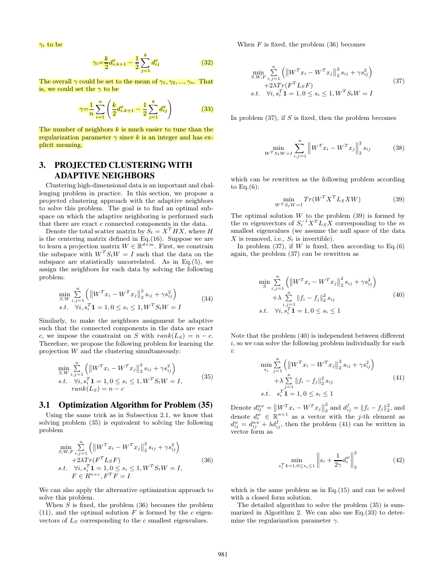Our goal is to construct a new similarity matrix to divide the data points into exact two clusters. From Fig. 1 we can easily ﬁnd the clustering eﬃciency of the proposed CAN method. In this ﬁgure, we set the color of the two clusters to be cyan and blue separately and let the width of the connecting line denote the learned similarity of two corresponding points. In the initial similarity matrix learned by Eq.(5), several pairs of points from diﬀerent clusters are connected. Whereas, after the learning by Eq.(7), there is not even a single line between these two clusters, which means that the proposed clustering method CAN can successfully partition the original data into two classes. 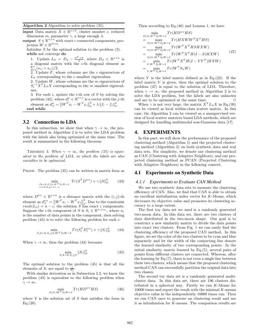The second toy data set is a randomly generated multi- cluster data. In this data set, there are 196 clusters dis- tributed in a spherical way. Firstly we run K-Means for 10000 times and report the result with the minimal K-means objective value in the independently 10000 times run. Then we run CAN once to generate an clustering result and use it as initialization for K-means. The comparison results are 982

1 0.5 0 −0.5 −1 1 0.5 0 −0.5 −1 1 0.5 0 −0.5 −1 −1 −0.5 0 0.5 1 1.5 −1 −0.5 0 0.5 1 1.5 −1 −0.5 0 0.5 1 1.5 (a) Original Data (b) Learnt Graph by Eq.(5) (c) Learnt Graph by Eq.(7) (CAN) Figure 1: Learned graph by CAN on the two-moon synthetic data. shown in Tab. 1 and Fig. 2. It is apparent that even after 10000 times run, the minimal K-means objective value and clustering accuracy obtained by K-means are far behind the result obtained by PCAN with only one run. Methods Acc%(min obj) Min obj K-Means 318.29 106.12 69.95 98.98 CAN Table 1: Clustering accuracy and minimal K-Means objective value on multi-cluster synthetic data sets. 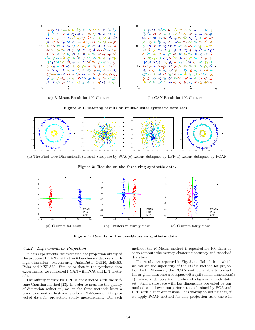ever, the PCAN method always behave well. The reason for this phenomenon is that PCA focus on the global structure thus fail immediately after the two clusters become close. While LPP pays more attention to the local structure, thus could achieve good performance when the two clusters are relatively close. But when the distance of these two clus- ters are fairly small, LPP is not capable any more. But our method, PCAN, lays more emphasis on the discriminative structure and thus keeps its projection quality all the time. 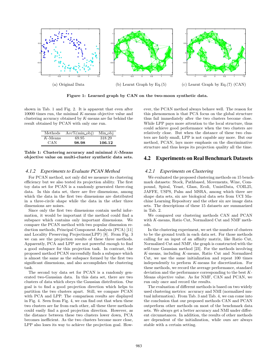4.2 Experiments on Real Benchmark Datasets 4.1.2 Experiments to Evaluate PCAN Method 4.2.1 Experiments on Clustering For PCAN method, not only did we measure its clustering eﬃciency but we also tested its projection ability. The ﬁrst toy data set for PCAN is a randomly generated three-ring data. In this data set, there are ﬁve dimensions, among which the data in the ﬁrst two dimensions are distributed in a three-circle shape while the data in the other three dimensions are noises. Since only the ﬁrst two dimensions contain useful infor- mation, it would be important if the method could ﬁnd a subspace which contains only important dimensions. We compare the PCAN method with two popular dimension re- duction methods, Principal Component Analysis (PCA) [11] and Locality Preserving Projections(LPP) [8]. From Fig. 3 we can see the projection results of these three methods. Apparently, PCA and LPP are not powerful enough to ﬁnd a good subspace for this projection task. In contrast, the proposed method PCAN successfully ﬁnds a subspace which is almost the same as the subspace formed by the ﬁrst two signiﬁcant dimensions, and also accomplishes the clustering task. The second toy data set for PCAN is a randomly gen- erated two-Gaussian data. In this data set, there are two clusters of data which obeys the Gaussian distribution. Our goal is to ﬁnd a good projection direction which helps to partition the two clusters apart. Still, we compare PCAN with PCA and LPP. The comparison results are displayed in Fig. 4. Seen from Fig. 4, we can ﬁnd out that when these two clusters are far from each other, all these three methods could easily ﬁnd a good projection direction. However, as the distance between these two clusters lower down, PCA becomes ineﬃcient. As the two clusters become more close, LPP also loses its way to achieve the projection goal. How- We evaluated the proposed clustering methods on 15 bench- mark datasets: Stock, Pathbased, Movements, Wine, Com- pound, Spiral, Yeast, Glass, Ecoli, UmistData, COIL25, JAFFE, USPS, Palm and MSRA, among which three are shape data sets, six are biological data sets from UCI Ma- chine Learning Repository and the other six are image data sets. The descriptions of these 15 datasets are summarized in Tab. 2. We compared our clustering methods CAN and PCAN with K-means, Ratio Cut, Normalized Cut and NMF meth- ods. In the clustering experiment, we set the number of clusters to be the ground truth in each data set. For those methods calling for an input of an aﬃnity matrix, like Ratio Cut, Normalized Cut and NMF, the graph is constructed with the self-tune Gaussian method [23]. For the methods involving K-means, including K-means, Ratio Cut and Normalized Cut, we use the same initialization and repeat 100 times independently to perform K-means for discretization. For these methods, we record the average performance, standard deviation and the performance corresponding to the best K- Means objective value. As for NMF, CAN and PCAN, we run only once and record the results. The evaluation of diﬀerent methods is based on two widely used clustering metrics: accuracy and NMI (normalized mu- tual information). From Tab. 3 and Tab. 4, we can come into the conclusion that our proposed methods CAN and PCAN outperform other methods on most of the benchmark data sets. We always get a better accuracy and NMI under diﬀer- ent circumstances. In addition, the results of other methods are dependent of the initialization, while ours are always stable with a certain setting. 983

15 10 5 0 0 1 0.5 0 −0.5 −1 15 10 5 0 0 5 10 15 5 10 15 (a) K-Means Result for 196 Clusters (b) CAN Result for 196 Clusters Figure 2: Clustering results on multi-cluster synthetic data sets. 2 1.5 1 0.5 0 −0.5 −1 −1.5 1.5 1 0.5 0 −0.5 −1 −1.5 1 0.5 0 −0.5 −1 −1.5 −1 −0.5 0 0.5 1 1.5 −2.5 −2 −1.5 −1 −0.5 0 0.5 1 1.5 2 −2 −1.5 −1 −0.5 0 0.5 1 1.5 2 −1.5 −1 −0.5 0 0.5 1 1.5 (a) The First Two Dimensions (b) Learnt Subspace by PCA (c) Learnt Subspace by LPP (d) Learnt Subspace by PCAN Figure 3: Results on the three-ring synthetic data. 8 6 4 2 0 −2 −4 −6 PCAN PCA LPP −10 −5 0 5 10 4 2 0 −2 −4 −6 −8 PCAN PCA LPP −5 0 5 6 4 2 0 −2 −4 −6 PCAN PCA LPP −5 0 5 (a) Clusters far away (b) Clusters relatively close (c) Clusters fairly close Figure 4: Results on the two-Gaussian synthetic data. 4.2.2 Experiments on Projection In this experiments, we evaluated the projection ability of the proposed PCAN method on 6 benchmark data sets with high dimension: Movements, UmistData, Coil20, Jaﬀe50, Palm and MSRA50. Similar to that in the synthetic data experiments, we compared PCAN with PCA and LPP meth- ods. The aﬃnity matrix for LPP is constructed with the self- tune Gaussian method [23]. In order to measure the quality of dimension reduction, we let the three methods learn a projection matrix ﬁrst and perform K-Means on the pro- jected data for projection ability measurement. For each method, the K-Means method is repeated for 100 times so as to compute the average clustering accuracy and standard deviation. The results are reported in Fig. 5 and Tab. 5, from which we can see the superiority of the PCAN method for projec- tion task. Moreover, the PCAN method is able to project the original data onto a subspace with quite small dimensions(c- 1), where c denotes the number of clusters in each data set. Such a subspace with low dimensions projected by our method would even outperform that obtained by PCA and LPP with higher dimensions. It is worthy to noting that, if we apply PCAN method for only projection task, the c in 984

分享到：

赞收藏

资料库

Clustering and Projected Clustering with Adaptive Neighbors论文.pdf

相关推荐

人工智能

热门标签

最新资料