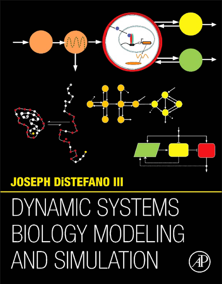
Front Cover
Dynamic Systems Biology Modeling and Simulation
Copyright Page
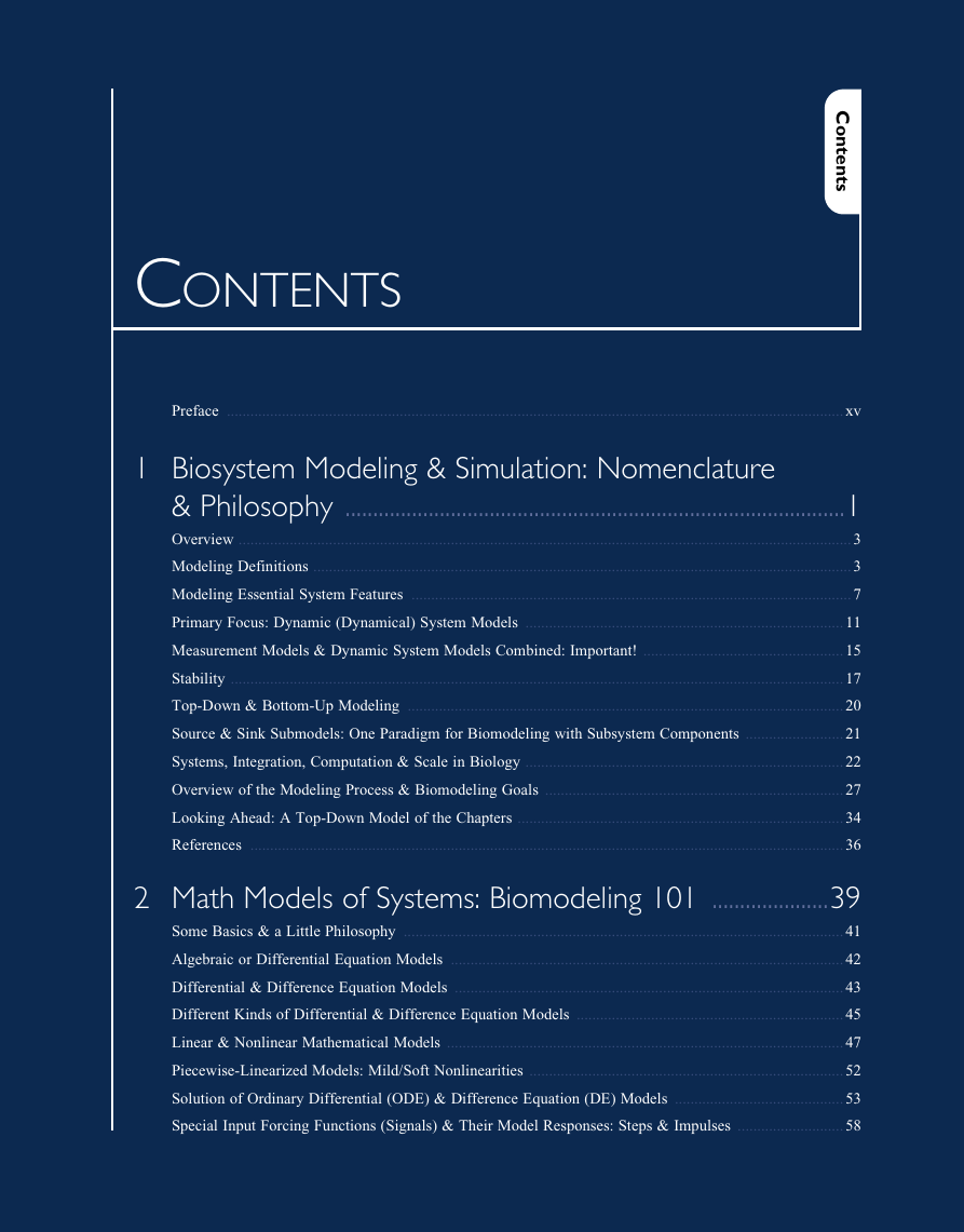
Contents
Preface to the First Edition
Pedagogical Struggles
Crystallizing and Focusing – My Way
In Other Words… & Other Didactic Devices
How to Use this Book in the Classroom
Acknowledgements
References
1 Biosystem Modeling & Simulation: Nomenclature & Philosophy
Overview
Modeling Definitions
Modeling Science
Modeling Essential System Features
Primary Focus: Dynamic (Dynamical) System Models
Deterministic vs. Stochastic Dynamic System Models
Markov Models
Measurement Models & Dynamic System Models Combined: Important!
Stability
Robustness & Fragility
Top-Down & Bottom-Up Modeling
Source & Sink Submodels: One Paradigm for Biomodeling with Subsystem Components
Systems, Integration, Computation & Scale in Biology
Systems Biology
Systems Physiology & Pharmacology
Multiscale Modeling
Bioinformatics
Computational Systems Biology & Computational Biology
Overview of the Modeling Process & Biomodeling Goals
Data-Driven Biomodeling: Structuring, Quantifying, Analyzing and Restructuring
The Biomodeling Process in Toto: A Philosophical Recap
Looking Ahead: A Top-Down Model of the Chapters
References
2 Math Models of Systems: Biomodeling 101
Some Basics & a Little Philosophy
Algebraic or Differential Equation Models
Differential & Difference Equation Models
Different Kinds of Differential & Difference Equation Models
Linear & Nonlinear Mathematical Models
Piecewise-Linearized Models: Mild/Soft Nonlinearities
Solution of Ordinary Differential (ODE) & Difference Equation (DE) Models
The Differential Operator D & Characteristic Equation: Characterizing Modes & Modal Dynamics of Linear ODE Models
Solution of Linear Time-Invariant (TI) ODEs
One Way to View ODE Solutions: Classical Approach
Convolution
The Transient & Steady State Responses: The Modern Systems Approach
Special Input Forcing Functions (Signals) & Their Model Responses: Steps & Impulses
The Unit Impulse Input: An Important Equivalence Property
State Variable Models of Continuous-Time Systems
Nonlinear (NL) State Variable Biomodels
Linear Time-Invariant (TI) Discrete-Time Difference Equations (DEs) & Their Solution
State Variable Models of Discrete-Time Systems
Linearity & Superposition
Laplace Transform Solution of ODEs
Four Key Properties of LT & ILT
Partial Fraction Expansions
Transfer Functions of Linear TI ODE Models
Transfer Function (TF) Matrix of an ODE
The Complex Plane: Pole-Zero Maps of Transfer Functions
More on System Stability
Stability of Linear TI Dynamic Systems
Looking Ahead
Exercises
References
3 Computer Simulation Methods
Overview
Initial-Value Problems
Graphical Programming of ODEs
Block Diagram Languages
Special Input Function Simulations
Impulse Inputs
Time-Delay Simulations
Multiscale Simulation and Time-Delays
Does Model Size Matter?
Normalization of ODEs: Magnitude- & Time-Scaling
Magnitude-Scaling ODEs
Time-Scaling ODEs
Numerical Integration Algorithms: Overview
The Taylor Series
Taylor Series Algorithms for Solving Ordinary Differential Equations
Computing Derivatives
Derivative Approximation Formulas
Local vs. Global Truncation Errors
Roundoff Errors
Computational/Numerical Stability
Self-Starting ODE Solution Methods
Euler Method
Runge–Kutta Methods
Main Features of R–K Methods
Fourth-Order Runge–Kutta Method
Stepwise Errors, Tolerances & Error Control
Algorithms for Estimating and Controlling Stepwise Precision
Runge–Kutta–Fehlberg (R–K–F)
Multistep Predictor–Corrector (P–C) Methods
Simple Multistep Formulas Based on Taylor Series
Taylor Series-Based Method Comparisons
Stiff ODE Problems
Stiff Solvers
How to Choose a Solver?
Solving Difference Equations (DEs) Using an ODE Solver
Other Simulation Languages & Software Packages
Math-Based Simulation Languages & Software
Special Purpose Simulation Packages in Biochemistry & Cell Biology
Stochastic Model Simulators
Two Population Interaction Dynamics Simulation Model Examples
Simpler & Linear Transcription/Translation Dynamics
Simple Predator–Prey Dynamics
Taking Stock & Looking Ahead
Exercises
4 Structural Biomodeling from Theory & Data: Compartmentalizations
Introduction
Compartmentalization: A First-Level Formalism for Structural Biomodeling
Basic Multicompartmental (MC) Model Formulation from Structural & Kinetic Data
Structural & Kinetic Data Complement Each Other
Input and Output Compartments First
More Compartments in More Organs
Handling Structural & Kinetic Data Mismatches: Caveat #1
Compartments, State Variables, Graphs, Pools & Chemical Species Defined
Mathematics of Multicompartmental Modeling from the Biophysics
The One-Compartment Model and Its Solution
Impulse-(Bolus)-Input Response: One-Compartment Model
Step-Input Response: One-Compartment Model
The Two-Compartment Model, its Forms, Properties & Solutions
Model Dynamics with Mass State Variables qi(t)
Model Dynamics with Concentration State Variables ci(t) ≡ qi(t)/Vi
Output Measurement Models
Model Outputs with Mass Measurements
Model Outputs with Concentration Measurements
Biosystem & Experiment Model Combined
Transfer Function Matrix for the Combined Biosystem & Experiment Model
Unit-Impulse Response from H(s)
Unit-Step Response: LT Solution
Steady State Solutions
Steady State Solutions for the Linear Two-Compartment Model
Nonlinear Multicompartmental Biomodels: Special Properties & Solutions
Nonlinear (NL) Compartment Model Building & Analysis
Dynamic System Nonlinear Epidemiological Models
SIS, SIR and SIRS Models
Epidemics & Reproduction Number R0
Compartment Sizes, Concentrations & the Concept of Equivalent Distribution Volumes
General n-Compartment Models with Multiple Inputs & Outputs
Model Dynamics
Output Measurements Model
The Constituent Compartmental Equations
Mammillary & Catenary Compartment Models
Data-Driven Modeling of Indirect & Time-Delayed Inputs
Signal Delay with Attenuation
Pools & Pool Models: Accommodating Inhomogeneities
Pool Models
Pool vs. Compartmental Model Applications: Flux-Balance & Cut-Set Analysis
Recap & Looking Ahead
Exercises
References
5 Structural Biomodeling from Theory & Data: Sizing, Distinguishing & Simplifying Multicompartmental Models
Introduction
Output Data (Dynamical Signatures) Reveal Dynamical Structure
What’s in the Box?
Multicompartmental Model Dimensionality, Modal Analysis & Dynamical Signatures
Multiexponential Impulse-Responses, Modes & Mode Parameters
Simplest Case: Distinct Eigenvalues (Distinct Exponents)
Dynamical Dimensionality: Establishing the Number of Compartments
Modes in Data ≡ Minimum Compartment Number
SISO Multiexponential Minimal Modeling: Some Answers & Insights
Composite Compartments: More Ambiguity & Insights
The Bigger Picture – Visible & Hidden Modes: Distinguishable & Indistinguishable Compartments (State Variables or Species)
Caveat #2 – Too Dynamically Simple?
Caveat #3 – Hidden Compartments?
Finding Modes (or Compartments) Visible in Output Data by Graphical Inspection
Automated Mode Detection Using Graph Theory Algorithms
Model Simplification: Hidden Modes & Additional Insights
State Variable Aggregation (Reduction): Transfer Functions Tell All
Biomodel Structure Ambiguities: Model Discrimination, Distinguishability & Input–Output Equivalence
*Algebra and Geometry of MC Model Distinguishability
Graph Properties & Geometric Rules
Automation: DISTING
Reducible, Cyclic & Other MC Model Properties
Tracers, Tracees & Linearizing Perturbation Experiments
Linearization of NL ODE Models
Linearized Output Measurement Model
The Complete Linearized Model
Recap and Looking Ahead
Exercises
References
6 Nonlinear Mass Action & Biochemical Kinetic Interaction Modeling
Overview
Kinetic Interaction Models
Linear & Monomolecular Interactions
Monomolecular Chemical Reactions
Monomolecular Irreversible
Monomolecular Reversible Conversion: Protein Folding and Unfolding
Nonlinear Bimolecular Reactions & Other Species Interactions
Molecular & Other Collisions: Combinatorial Product Laws
Energetics, Reaction Activation & Transformation
Volume & Temperature Effects
Law of Mass Action
Reaction Rate Equations
Reversible Reactions & Dynamic Equilibrium
Reaction Dynamics in Open Biosystems
Enzymes & Enzyme Kinetics
Substrate–Enzyme Interactions: Michaelis–Menten Theory
The Quasi-Steady State Assumption (QSSA) & the M–M Approximate Equations
M–M QSSA Equation Extremes
M–M QSSA Equation Representations, Transformations & Quantification
Total Quasi-Steady State Assumption (tQSSA): When the QSSA is not Valid
Summary Equations & Conditions for the QSSA and First-Order tQSSA
Enzymatic Regulation of Biochemical Pathways
Enzymes & Introduction to Metabolic and Cellular Regulation
A Simple Competitive Reaction: One Enzyme & Two Substrates
Local Regulation by Enzymatic Activation–Deactivation
*More Complex Regulation: Cooperativity and Allosterism
*Allosterism Modeling
Other Allosterism Models & Summary Remarks
Exercises
Extensions: Quasi-Steady State Assumption Theory
*Classic Michaelis–Menten Theory
*Modern Quasi-Steady State Assumption (QSSA) Analysis & a Scaling Lesson
References
7 Cellular Systems Biology Modeling: Deterministic & Stochastic
Overview
Enzyme-Kinetics Submodels Extrapolated to Other Biomolecular Systems
Simple Models of Production Rate Regulation
Hill Function Regulation Models
Ligand–Receptor Interactions & Drug Dynamics
Pharmacodynamic Stimulus & Inhibitory Approximation Functions
Coupled-Enzymatic Reactions & Protein Interaction Network (PIN) Models
When the tQSSA is More Appropriate than the QSSA
Production, Elimination & Regulation Combined: Modeling Source, Sink & Control Components
The Stoichiometric Matrix N
Special Purpose Modeling Packages in Biochemistry, Cell Biology & Related Fields
Stochastic Dynamic Molecular Biosystem Modeling
When a Stochastic Model is Preferred
*Stochastic Process Models & the Gillespie Algorithm
Nomenclature & Equations
The Chemical Master Equation
The Gillespie Algorithm & Variants
Algorithm Properties
*Stochastic Model Analysis: Ensemble Statistics
Exercises
References
8 Physiologically Based, Whole-Organism Kinetics & Noncompartmental Modeling
Overview
Physiologically Based (PB) Modeling
Nomenclature
Simplified Vascular & Tissue Physiology & Anatomy for PB Modeling
Blood & Lymph Vessels, their Constituents & Tissue Distributions
Structuring & Parameterizing a PB Model
Diagram Notation
PBPK (PBPD, PBTK) Model Organs & Compartments
Plasma vs. Blood Concentrations & Flow Rates
Distribution Dynamics of Blood Constituents in Tissues
PBPK Model Parameters
Dynamical Equations of PB Models
Simplest Single-Organ Model
Permeability-Limited Two-Subcompartment (PLT) Organ Model
Three-Compartment Organ in a Whole-Body Model
Two-Region Asymptotically Reduced (TAR) Models
PB Examples in Toxicology
Allometric Scaling in PB Models
Experiment Design Issues in Kinetic Analysis (Caveats)
Linear vs. Nonlinear (NL)
Time-varying vs. Time-Invariant/Stationary
Whole-Organism Parameters: Kinetic Indices of Overall Production, Distribution & Elimination
Measures of Elimination & Production & their Data-Driven Models
Plasma Clearance Rate (PCR)
PCR Experiment Designs
Other Clearance Rates: UCR & FCR
Distribution Volume, Partition Coefficient & Pool Size Relationships
Residence Times
Whole-Organism Parameter Relationships
Half-Lives
Noncompartmental (NC) Biomodeling & Analysis (NCA)
Noncompartmental Analysis Formulas
Noncompartmental Parameters from Multiexponential Models
Bioavailability & Bioequivalence in Pharmacology
Noncompartment Model Structure Problems
The Equivalent Sink Problem: NC Model Structural Constraint #1
The Equivalent Source Problem: NC Model Structural Constraint #2
Exchangeable or Circulating Masses & Volumes as NC Parameter Bounds
Summarizing Noncompartmental Analysis (NCA) Applicability
Bounds for Whole-Organ System Parameters from NCA
NC Model Structure Errors & Some Consequences
Very Limited Compartmental Equivalents of Noncompartmental Models
NC versus MC Modeling: No Easy Choice
Recap & Looking Ahead
Exercises
References
9 Biosystem Stability & Oscillations
Overview/Introduction
Biosystem Stability
Oscillations in Biology
Stability of NL Biosystem Models
Phase Space Geometry
Stability, Equilibrium Points, Steady State Solutions & Nullclines
Stability Classifications
Stability of Linear System Models
Local Nonlinear Stability via Linearization
Bifurcation Analysis
Other Bifurcation Types
Oscillations in Biology
Harmonic Oscillations
Limit Cycle Oscillations
Oscillations & the Selkov Model of Glycolysis
Oscillations & the Brusselator Model
Other Complex Dynamical Behaviors
Chaos
Complex Dynamic System Behavior & Chaos for the Discrete-Time Logistic Population Growth Model
The Lorenz Model & Lorenz Attractor
Concluding Remarks About Chaos & Complexity
Nonlinear Modes
Nonlinear Modes in Systems Biology
Recap & Looking Ahead
Exercises
References
10 Structural Identifiability
Introduction
Model/Parameter Quantification & Identifiability (SI & NI) Defined
Structural Identifiability (SI) in the Large
Historical Perspective
Basic Concepts
Complete Biosystem Model: Constraints as Well as Inputs & Outputs Included
Transfer Functions & SI
Preliminary Definitions
Structural Invariants
Ambiguities
Multiple Inputs
Formal Definitions: Constrained Structures, Structural Identifiability & Identifiable Combinations
Unidentifiable Models
Interval Identifiability & Parameter Interval Analysis
Parameter Bounds & Quasiidentifiability Conditions
Bounds for n-Compartment Models
Bounds on Equivalent Distribution Volumes
Quasiidentifiability Conditions
Informational Limitations in Unidentifiable Models
SI Under Constraints: Interval Identifiability with Some Parameters Known
General Catenary & Mammillary Model Equations
Feasible Parameter Ranges (Subspace) for Equality Constraints
Models with Infeasible or Redundant Constraints
The Constrained Parameter Bounding Algorithms
Catenary Model
Mammillary Model
Joint Submodel Parameters: Another Approach to Interval Identifiability
SI Analysis of Nonlinear (NL) Biomodels
Prolog and Overview
SI Analysis by Taylor Series
SI Analysis by Symbolic Differential Algebra (DA)
What’s Next?
Exercises
References
11 Parameter Sensitivity Methods
Introduction
Sensitivity to Parameter Variations: The Basics
Relative Sensitivity of Outputs & Functions of Outputs to Parameter Variations
Multiple Outputs & Parameters
State Variable Sensitivities to Parameter Variations
Total (Global) & First-Order (Local, Linear) Variations & Sensitivities
First-Order (Local, Linear) Variations & Sensitivities
Local State Variable Sensitivities
Some Notable Features of State Variable Sensitivity Functions
*The Canonical Sensitivity System
Output Sensitivities to Parameter Variations
Some Notable Features of Output Sensitivity Functions
Time-Averaged Relative Output Sensitivity Functions
Sensitivity Measures of Model Quantification Results (Robustness)
*Output Parameter Sensitivity Matrix & Structural Identifiability
Key Output Sensitivity Matrix–SI Relationships
*Global Parameter Sensitivities
Recap & Looking Ahead
Exercises
References
12 Parameter Estimation & Numerical Identifiability
Biomodel Parameter Estimation (Identification)
Model Quantification by any Other Name
Model Fitting
Parameter Estimation, Robustness and Sensitivity
What/Which Parameters are Estimated?
Robustness, Sensitivity & Parameter Estimation
Different Quantification Approaches
Direct vs. Indirect Parameter Estimation
Indirect Parameter Estimation
Linear Constant-Coefficient Models: Multiexponential Response Approach
Linear & Nonlinear in the Parameters Models
Residual Errors & Parameter Optimization Criteria
Residual Output Errors for Discrete-Time Measurements
Least-Squares (LS) Criteria
Weighted Least-Squares (WLS) or Residual Sum of Squares (WRSS) Criteria
*WLS for More Than One Output: y(t)=[y1(t) ··· ym(t)]T
Extended Weighted Least Squares (EWLS)
Maximum Likelihood (ML)
Parameter Optimization Methods 101: Analytical and Numerical
The Calculus of Linear Least Squares
The Curve-Peeling (or Stripping) Method for Exponential Curve Fitting
Iterative Search Algorithms, Local & Global
Local Search
*Global Search
Parameter Estimation Quality Assessments
Numerical (a Posteriori, Practical) Identifiability (NI): Distinguishing the Practical from the Possible
Output Sensitivity Matrix & Numerical Identifiability
Parameter Variances, Covariance/Correlation Matrices & Identifiability Relationships
Parameter Standard Errors (SEs) & Standard Deviations (SDs)
VAR(pi) & CORR(pipj) for Identifiability Testing
COV(p)≅H(p) from the Hessian Matrix
COV(p)≥F−1(p) from the Fisher Information Matrix
The Cramér–Rao Theorem
Residual Mean Square (RMS) Error & COV(p*) for Unweighted Regression
Covariance & Fisher Information Matrices for Functions b(p) of p
*COV(p) by Stochastic Monte Carlo Simulation
Robustness and Sensitivities from COV(p)
Other Biomodel Quality Assessments
Goodness-of-Fit Criteria & Figures of Merit – Subjective & Statistical
The “Eyeball” Test: Visual Inspection
Analysis of Residuals
Appropriate Weighting of the Data
Independence of Residual Errors
Gaussian Distribution & Independence of Residuals
Recap and Looking Ahead
Exercises
References
13 Parameter Estimation Methods II: Facilitating, Simplifying & Working With Data
Overview
Prospective Simulation Approach to Model Reliability Measures
Structurally Identifiable or Not
Structurally Identifiable NL & Numerically Identifiable (NI) or Not NI
Variances, Covariances & Correlations
Input–Output Models
Constraint-Simplified Model Quantification
Model Reparameterization & Quantifying the Identifiable Parameter Combinations
Reparameterized Model Statistics with Noisy Data
Covariance COV(b) in Terms of Identifiable Parameter Combinations c
Combos, Noisy Data & Parameter Equality Constraint Effects
The Forcing-Function Method
Multiexponential (ME) Models & Use as Forcing Functions
Model Fitting & Refitting With Real Data
Recap and Looking Ahead
Exercises
References
14 Biocontrol System Modeling, Simulation, and Analysis
Overview
Physiological Control System Modeling
Neuroendocrine Physiological System Models
Models in the Literature
Anatomy of a Neuroendocrine Model
Neuroendocrine Regulation of Thyroid Hormones (TH) in the Human: A Feedback Control System (fbcs) Simulation Model
Overall Block Diagram
Data
Equations
Brain Submodels
TH Submodels
T3 & T4 (=TH) Distribution and Elimination (D&E) Submodel
Gut Absorption Submodel – Needed for Representing Oral Dosing
Preliminary Quantification
Closed-Loop Quantification
Structural Modeling & Analysis of Biochemical & Cellular Control Systems
Open- vs. Closed-Loop Biochemical Reaction Dynamics
Open-Loop Model
Closed-Loop Model
Approximate QSSA Model Solution is Qualitatively Different (Wrong)
Transient and Steady-State Biomolecular Network Modeling
Modeling Complete Dynamics
Different ODE Model Forms
Metabolism and Steady State Flux Balance Analysis (FBA)
Optimizing Steady-State Fluxes
Experiment Design for FBA by Cutset Analysis
Elementary Mode and Extreme Pathway Analysis
Metabolomics
Metabolomics in Synthetic and Mammalian Biology
Metabolic Control Analysis (MCA)
Sensitivity Functions of Metabolic Control Analysis
Properties of Metabolic Control and Elasticity Coefficients
Control Coefficient Constraints
Control and Elasticity Connectivity Properties
Recap and Looking Ahead
Exercises
References
15 Data-Driven Modeling and Alternative Hypothesis Testing
Overview
Let the Data Speak First
Formalizing the Modeling Process Based on the Data
Statistical Criteria for Discriminating Among Alternative Models
Multiexponential/Multicompartmental Model Discrimination: How Many Modes?
F-test of Significance
Testing Estimates of Exponential Coefficients Ai
Akaike Information Criterion (AIC)
The Schwarz Criterion (SC or BIC)
Macroscale and Mesoscale Models for Elucidating Biomechanisms
Minimal Macroscale Disease Dynamics Models: Treatment of Viral Infections
Mesoscale Mechanistic Models of Biochemical/Cellular Control Systems
What Signals Control Frog Egg Maturation (Cellular Decision-Making)?
Testing Six Alternative Steroid Dynamics Hypotheses Using Biochemistry, PK, PD, and Pharmacogenomic Data
Pedagogic Perspective on Structural Assumptions
Testing Manganese Brain Entry Pathway Hypotheses from Quantified Distribution Dynamics of Multiorgan Rat Data
Model Structure
Data, Data-Driven Structural Assumptions and Equations
Model Quantification
Candidate Models for p53 Regulation
What Does p53 Do? – Modeler’s Perspective
p53 Multifeedback Regulation
Other Regulatory Factors and Variables
Different p53 Models are OK
p53 Oscillations and Models of How They Arise
Stochastic p53 Models
Different Structures for Different Inputs
A 4-State Variable Alternative Model for p53–Mdm2–MdmX Signaling
Model Input
Model Output Measurement Equations
Parameter Relationships from Steady State Constraints
Structural Parameter Identifiability
Initial Parameter Estimation and Numerical Identifiability
Preliminary p53 Signaling Model Stability Analysis
Recap and Looking Ahead
Exercises
References
16 Experiment Design and Optimization
Overview
A Formal Model for Experiment Design
Design-Degrees-of-Freedom
Input–Output Experiment Design from the TF Matrix
Experiment Design by Exhaustive SI Analysis of the General 2-Compartment Model
Experiment Design by Exhaustive SI Analysis of a 6-Compartment Biomodel
Feasible Experiments
Transfer Function Matrix
Identifiability Analysis for Each Hij
Identifiability Analysis for Combinations of Hij: SI from Multiple Experiments
Alternative Combinations of Physiological Experiments
Aggregated Measurements
Practical Alternatives via External Monitoring
Graphs and Cutset Analysis for Experiment Design
Some Cutset Theory and Applications
Basics of Cutset Analysis
Procedural Rules for Experiment Design
Parameter kji from Two or Three Steady State Experiments
Algorithms for Optimal Experiment Design
Scalar Optimization Functions of F
Optimal Sampling Schedule Design
Sequential Optimal Experiment Design
OSS Design Software
OSS Design Applied in Practice
Sequential Designs
Optimally Quantified Model
Recap and Looking Ahead
Exercises
References
17 Model Reduction and Network Inference in Dynamic Systems Biology
Overview
Local and Global Parameter Sensitivities
Model Reduction Methodology
Parameter Ranking
Simple RMS Metric for Local Sensitivity-Based Parameter Ranking
Geometric Metric for Parameter Ranking
Added Benefits: State Variables to Measure and Parameters to Estimate
Reducing a Model of NFκB Signaling Dynamics
Parameter Ranking Metrics Based on Optimizing the Fisher Information Matrix F
Reducing a Model of Interleukin-6 (IL-6) Signaling Dynamics
Reducing an Overparameterized (OPM) Model of p53 Signaling Dynamics
Global Sensitivity Analysis (GSA) Algorithms
Weighted-Average of Local Relative Sensitivities (WAR) Spy=(∂y/y)/(∂p/p)
The WAR Approximate GSA Algorithm
Multi-Parametric Sensitivity Analysis
MPSA Algorithm
What’s Next?
Exercises
References
Appendix A: A Short Course in Laplace Transform Representations & ODE Solutions
Transform Methods
Laplace Transform Representations and Solutions
Two-Step Solutions
Key Properties of the Laplace Transform (LT) & its Inverse (ILT)
Short Table of Laplace Transform Pairs
Laplace Transform Solution of Ordinary Differential Equations (ODEs)
Partial Fraction Expansions
Inverse Transforms Using Partial Fraction Expansions
References
Appendix B: Linear Algebra for Biosystem Modeling
Overview
Matrices
Vector Spaces (V.S.)
Linear Equation Solutions
Minimum Norm & Least Squares Pseudoinverse Solutions of Linear Equations
Measures & Orthogonality
Matrix Analysis
Matrix Norms
Matrix Calculus
Computation of f(A), an Analytic Function of a Matrix
Special Case (a): A=Λ
Special Case (b): Spectral Representation of A
The Cayley–Hamilton Theorem: An Alternative Method for Computing f(A)
A Combination of the Previous Two Methods for Distinct Eigenvalues
For Nondistinct (Repeated) Eigenvalues
Matrix Differential Equations
Singular Value Decomposition (SVD) & Principal Component Analysis (PCA)
Singular Value Decomposition (SVD)
Some Properties of the SVD
Principal Component Analysis (PCA)
PCA from SVD
Data Reduction & Geometric Interpretation
References
Appendix C: Input–Output & State Variable Biosystem Modeling: Going Deeper
Inputs & Outputs
Dynamic Systems, Models & Causality
Input–Output (Black-Box) Models
Time-Invariance (TI)
Continuous Linear System Input–Output Models
Transfer Function (TF) Matrix for Linear TI Input–Output Models
Structured State Variable Models
State of a System S or Model M
State Variable Models from Input–Output (I–O) Models
Dynamic State Variable ODE Models for Continuous Systems
Complete Dynamic System Models: Constrained Structures
Linear TI State Variable Models
Input–Output TF Matrix for a State Variable Model
Discrete-Time Dynamic System Models
Discrete-Time Input–Output Models
The Sampled or z-Transfer Function
Discrete-Time State Variable Models
Sampled Input–Output Transfer Function Matrix
Composite Input–Output and State Variable Models
Composite Input–Output Models
Composite State Variable Models
State Transition Matrix for Linear Dynamic Systems
Input–Output Model Solutions
State Variable Model Solutions
Continuous Case
Intuitive Explanation of Φ
Time-Invariant Case
The Adjoint Dynamic System
Equivalent Dynamic Systems: Different Realizations of State Variable Models – Nonuniqueness Exposed
Key Properties of Equivalent System Models
Example C.1
Discrete-Time State Variable Models
Illustrative Example: A 3-Compartment Dynamic System Model & Several Discretized Versions of It
Discretization & Sampled-Data Representations of the 3-Compartment Model
Pulse-Train Inputs
Impulse-Train Inputs
Discretized ARMA Model with Impulse-Train Input
Transforming Input–Output Data Models into State Variable Models: Generalized Model Building
Time-Invariant Realizations
SISO Models
Appendix D: Controllability, Observability & Reachability
Basic Concepts and Definitions
Controllability
Observability
Observability and Controllability of Linear State Variable Models
Linear Time-Varying Models
Controllability Criterion
Observability Criterion
Linear Time-Invariant Models
Practical Controllability and Observability Conditions
Output Controllability
Time-Invariant (TI) Models
TI State Variable Models
Output Function Controllability
Reachability
Constructibility
Controllability and Observability with Constraints
Positive Controllability
Relative Controllability (Reachability)
Conditional Controllability
Structural Controllability and Observability
Observability and Identifiability Relationships
Controllability and Observability of Stochastic Models
References
Appendix E: Decomposition, Equivalence, Minimal & Canonical State Variable Models
Realizations (Modeling Paradigms)
The Canonical Decomposition Theorem
How to Decompose a Model
Controllability and Observability Tests Using Equivalent Models
SISO Models
Case 1
Case 2 (SISO)
MIMO Models
Case 1
Case 2
Minimal State Variable (ODE) Models from I–O TFs (Data)
Minimal SISO State Variable Models
Minimal MIMO State Variable Models
Canonical State Variable (ODE) Models from I–O Models (Data)
Companion Canonical Models
Canonical State Variable Models for More General SISO TFs
Jordan-Canonical State Variable Models for N(s)/D(s)
Controllable Canonical State Variable Models for N(s)/D(s)
Observable Canonical State Variable (ODE) Models for N(s)/D(s)
Observable and Controllable Canonical Forms from Arbitrary State Variable Models Using Equivalence Properties
References
Appendix F: More on Simulation Algorithms & Model Information Criteria
Additional Predictor-Corrector Algorithms
Modified Euler Second-Order Predictor and Corrector Formulas
An Iterative-Implicit Predictor–Corrector Algorithm
Noniterative, Predictor–Modifier–Corrector (P–M–C) Algorithms
Truncation Error Estimation
A Predictor-Modifier Corrector Algorithm Exemplified
The Backward-Euler Algorithm for Stiff ODEs
Derivation of the Akaike Information Criterion (AIC)
The AIC for Nonlinear Regression
Case 1 – σi2 Known
Case 2 – The Data Variances σi2≡ksi2 are Known Up to a Proportionality Constant k
The Stochastic Fisher Information Matrix (FIM): Definitions & Derivations
FIM for Multioutput Models
Index






 2023年江西萍乡中考道德与法治真题及答案.doc
 2012年重庆南川中考生物真题及答案.doc
 2013年江西师范大学地理学综合及文艺理论基础考研真题.doc
 2020年四川甘孜小升初语文真题及答案I卷.doc
 2020年注册岩土工程师专业基础考试真题及答案.doc
 2023-2024学年福建省厦门市九年级上学期数学月考试题及答案.doc
 2021-2022学年辽宁省沈阳市大东区九年级上学期语文期末试题及答案.doc
 2022-2023学年北京东城区初三第一学期物理期末试卷及答案.doc
 2018上半年江西教师资格初中地理学科知识与教学能力真题及答案.doc
 2012年河北国家公务员申论考试真题及答案-省级.doc
 2020-2021学年江苏省扬州市江都区邵樊片九年级上学期数学第一次质量检测试题及答案.doc
 2022下半年黑龙江教师资格证中学综合素质真题及答案.doc