聚类评估指标分析.pdf

发布时间：2022-06-19 发布人：admin 分类：说明书资料大小：0.36M 资料格式：pdf 举报版权申诉

3e467537-0942-40cd-87e2-793eb7f780f5.pdf-第1页.png

第1页 / 共34页

3e467537-0942-40cd-87e2-793eb7f780f5.pdf-第2页.png

第2页 / 共34页

3e467537-0942-40cd-87e2-793eb7f780f5.pdf-第3页.png

第3页 / 共34页

3e467537-0942-40cd-87e2-793eb7f780f5.pdf-第4页.png

第4页 / 共34页

3e467537-0942-40cd-87e2-793eb7f780f5.pdf-第5页.png

第5页 / 共34页

3e467537-0942-40cd-87e2-793eb7f780f5.pdf-第6页.png

第6页 / 共34页

3e467537-0942-40cd-87e2-793eb7f780f5.pdf-第7页.png

第7页 / 共34页

3e467537-0942-40cd-87e2-793eb7f780f5.pdf-第8页.png

第8页 / 共34页

文本预览

Clustering Indices Bernard Desgraupes University Paris Ouest Lab Modal’X April 2013 Contents 1 Internal clustering criteria 1.2 1.1 Algebraic background and notations . . . . . . . . . . . . . . . . 1.1.1 Total dispersion . . . . . . . . . . . . . . . . . . . . . . . 1.1.2 Within-group scatter . . . . . . . . . . . . . . . . . . . . . 1.1.3 Between-group scatter . . . . . . . . . . . . . . . . . . . . 1.1.4 Pairs of points . . . . . . . . . . . . . . . . . . . . . . . . Internal indices . . . . . . . . . . . . . . . . . . . . . . . . . . . . 1.2.1 The Ball-Hall index . . . . . . . . . . . . . . . . . . . . . 1.2.2 The Banfeld-Raftery index . . . . . . . . . . . . . . . . . 1.2.3 The C index . . . . . . . . . . . . . . . . . . . . . . . . . 1.2.4 The Calinski-Harabasz index . . . . . . . . . . . . . . . . 1.2.5 The Davies-Bouldin index . . . . . . . . . . . . . . . . . . 1.2.6 The Det Ratio index . . . . . . . . . . . . . . . . . . . . . 1.2.7 The Dunn index . . . . . . . . . . . . . . . . . . . . . . . 1.2.8 The Baker-Hubert Gamma index . . . . . . . . . . . . . . 1.2.9 The GDI index . . . . . . . . . . . . . . . . . . . . . . . . 1.2.10 The G plus index . . . . . . . . . . . . . . . . . . . . . . . 1.2.11 The Ksq DetW index . . . . . . . . . . . . . . . . . . . . 1.2.12 The Log Det Ratio index . . . . . . . . . . . . . . . . . . 1.2.13 The Log SS Ratio index . . . . . . . . . . . . . . . . . . . 1.2.14 The McClain-Rao index . . . . . . . . . . . . . . . . . . . 1.2.15 The PBM index . . . . . . . . . . . . . . . . . . . . . . . 1.2.16 The Point-Biserial index . . . . . . . . . . . . . . . . . . . 1.2.17 The Ratkowsky-Lance index . . . . . . . . . . . . . . . . . 1.2.18 The Ray-Turi index . . . . . . . . . . . . . . . . . . . . . 1.2.19 The Scott-Symons index . . . . . . . . . . . . . . . . . . . 1.2.20 The SD index . . . . . . . . . . . . . . . . . . . . . . . . . 1.2.21 The S Dbw index . . . . . . . . . . . . . . . . . . . . . . . 1.2.22 The Silhouette index . . . . . . . . . . . . . . . . . . . . . 1.2.23 The Tau index . . . . . . . . . . . . . . . . . . . . . . . . 1.2.24 The Trace W index . . . . . . . . . . . . . . . . . . . . . 1.2.25 The Trace WiB index . . . . . . . . . . . . . . . . . . . . 1 3 3 3 4 6 6 7 7 9 9 9 10 10 10 11 12 13 13 13 13 13 14 14 15 15 16 16 17 18 18 19 19

Package clusterCrit for R 1.2.26 The Wemmert-Gan¸carski index . . . . . . . . . . . . . . . 1.2.27 The Xie-Beni index . . . . . . . . . . . . . . . . . . . . . . 1.3 Choice of the best partition . . . . . . . . . . . . . . . . . . . . . 2 External comparison indices 2.1 Notation . . . . . . . . . . . . . . . . . . . . . . . . . . . . . . . . 2.2 Precision and recall coeﬃcients . . . . . . . . . . . . . . . . . . . 2.3 Indicator variables . . . . . . . . . . . . . . . . . . . . . . . . . . 2.4 External indices deﬁnition . . . . . . . . . . . . . . . . . . . . . . 2.4.1 The Czekanowski-Dice index . . . . . . . . . . . . . . . . 2.4.2 The Folkes-Mallows index . . . . . . . . . . . . . . . . . . 2.4.3 The Hubert ˆΓ index . . . . . . . . . . . . . . . . . . . . . 2.4.4 The Jaccard index . . . . . . . . . . . . . . . . . . . . . . 2.4.5 The Kulczynski index . . . . . . . . . . . . . . . . . . . . 2.4.6 The McNemar index . . . . . . . . . . . . . . . . . . . . . 2.4.7 The Phi index . . . . . . . . . . . . . . . . . . . . . . . . 2.4.8 The Rand index . . . . . . . . . . . . . . . . . . . . . . . 2.4.9 The Rogers-Tanimoto index . . . . . . . . . . . . . . . . . 2.4.10 The Russel-Rao index . . . . . . . . . . . . . . . . . . . . 2.4.11 The Sokal-Sneath indices . . . . . . . . . . . . . . . . . . 3 Usage of the clusterCrit package 3.1 Available commands . . . . . . . . . . . . . . . . . . . . . . . . . 3.2 Examples of use . . . . . . . . . . . . . . . . . . . . . . . . . . . . 3.3 Benchmark . . . . . . . . . . . . . . . . . . . . . . . . . . . . . . Bibliography 2 20 20 22 22 23 23 24 24 24 25 25 25 25 25 26 26 26 26 26 27 27 28 30 33

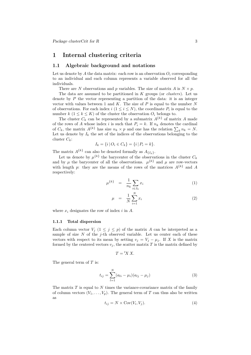
Package clusterCrit for R 3 1 Internal clustering criteria 1.1 Algebraic background and notations Let us denote by A the data matrix: each row is an observation Oi corresponding to an individual and each column represents a variable observed for all the individuals. There are N observations and p variables. The size of matrix A is N × p. The data are assumed to be partitioned in K groups (or clusters). Let us denote by P the vector representing a partition of the data: it is an integer vector with values between 1 and K. The size of P is equal to the number N of observations. For each index i (1 ≤ i ≤ N ), the coordinate Pi is equal to the number k (1 ≤ k ≤ K) of the cluster the observation Oi belongs to. The cluster Ck can be represented by a submatrix A{k} of matrix A made of the rows of A whose index i is such that Pi = k. If nk denotes the cardinal k nk = N . Let us denote by Ik the set of the indices of the observations belonging to the cluster Ck: of Ck, the matrix A{k} has size nk × p and one has the relation Ik = {i| Oi ∈ Ck} = {i| Pi = k}. The matrix A{k} can also be denoted formally as A{Ik}. Let us denote by µ{k} the barycenter of the observations in the cluster Ck and by µ the barycenter of all the observations. µ{k} and µ are row-vectors with length p: they are the means of the rows of the matrices A{k} and A respectively: N i∈Ik i=1 µ{k} = µ = 1 nk 1 N xi xi (1) (2) where xi designates the row of index i in A. 1.1.1 Total dispersion Each column vector Vj (1 ≤ j ≤ p) of the matrix A can be interpreted as a sample of size N of the j-th observed variable. Let us center each of these vectors with respect to its mean by setting vj = Vj − µj. If X is the matrix formed by the centered vectors vj, the scatter matrix T is the matrix deﬁned by T = tX X. The general term of T is: N l=1 tij = (ali − µi)(alj − µj) (3) The matrix T is equal to N times the variance-covariance matrix of the family of column vectors (V1, . . . , Vp). The general term of T can thus also be written as tij = N × Cov(Vi, Vj). (4)

Package clusterCrit for R 4 In particular, the diagonal terms are N times the variances of the vectors Vi: tii = N × Var(Vi). One can also write: tij = t(Vi − µi)(Vj − µj) (5) (6) where, by a slight abuse of notation, µi and µj are here identiﬁed with the vectors µi1 and µj1 respectively. The scatter matrix is a square symmetric matrix of size p× p. As it is of the form tX X, the quadratic form it represents is positive semi-deﬁnite. Indeed, if one takes any vector v in Rp: tvT v = tvtX Xv = t(Xv) (Xv) = ||Xv||2 ≥ 0 (7) In particular, the eigenvalues and the determinant of the scatter matrix are also greater than or equal to 0. If N > p and if the matrix X has maximal rank p, the form is in fact positive deﬁnite. The total scattering TSS (total sum of squares) is the trace of the matrix T : T SS = Tr(T ) = N Var(Vj) (8) p j=1 Geometric interpretation: let us denote by M1, . . . , MN the points of the space Rp representing all the observations: the coordinates of Mi are the coef- ﬁcients of the i-th row of the datat matrix A. Similarly, let us denote by G the barycenter of these points: its coordinates are the coeﬃcients of the vector µ. One can easily prove the following relations: N i=1 1 N i

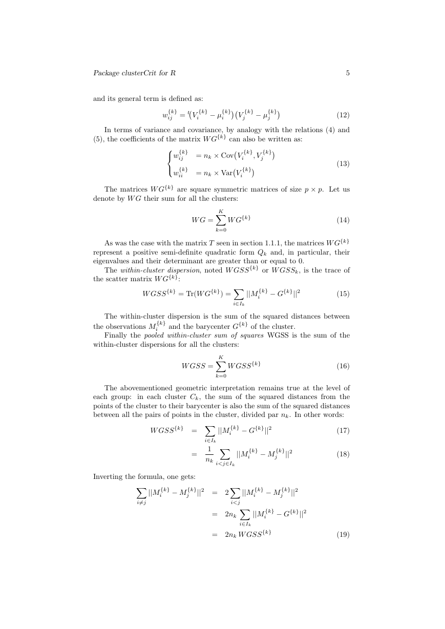
Package clusterCrit for R and its general term is deﬁned as: {k} j − µ {k} j 5 (12) In terms of variance and covariance, by analogy with the relations (4) and (5), the coeﬃcients of the matrix W G{k} can also be written as: w {k} ij = tV w {k} ij {k} ii w {k} i {k} i − µ V = nk × CovV = nk × VarV K W G = W G{k} k=0 {k} , V j {k} i {k} i The matrices W G{k} are square symmetric matrices of size p × p. Let us denote by W G their sum for all the clusters: (13) (14) (17) (18) (19) As was the case with the matrix T seen in section 1.1.1, the matrices W G{k} represent a positive semi-deﬁnite quadratic form Qk and, in particular, their eigenvalues and their determinant are greater than or equal to 0. The within-cluster dispersion, noted W GSS{k} or W GSSk, is the trace of the scatter matrix W G{k}: W GSS{k} = Tr(W G{k}) = ||M {k} i − G{k}||2 (15) i∈Ik The within-cluster dispersion is the sum of the squared distances between the observations M {k} i and the barycenter G{k} of the cluster. Finally the pooled within-cluster sum of squares WGSS is the sum of the within-cluster dispersions for all the clusters: W GSS = W GSS{k} (16) K k=0 The abovementioned geometric interpretation remains true at the level of each group: in each cluster Ck, the sum of the squared distances from the points of the cluster to their barycenter is also the sum of the squared distances between all the pairs of points in the cluster, divided par nk. In other words: W GSS{k} = = Inverting the formula, one gets: {k} j {k} i − M ||M i=j ||2 = 2 i∈Ik 1 nk i

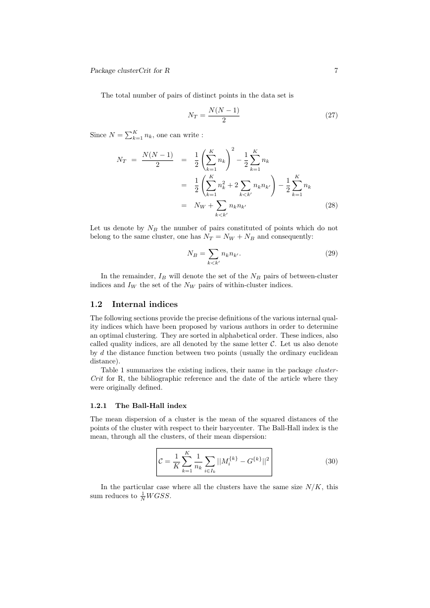
Package clusterCrit for R 6 1.1.3 Between-group scatter The between-group dispersion measures the dispersion of the clusters between each other. Precisely it is deﬁned as the dispersion of the barycenters G{k} of each cluster with respect to the barycenter G of the whole set of data. Let us denote by B the matrix formed in rows by the vectors µ{k} − µ, each one being reproduced nk times (1 ≤ k ≤ K). The between-group scatter matrix is the matrix BG = tB B. The general term of this matrix is: The between-group dispersion BGSS is the trace of this matrix: (20) (21) (22) K k=1 bij = nk(µ {k} j − µj) {k} i − µi)(µ K K K p nk k=1 k=1 nk k=1 j=0 t(µ{k} − µ)(µ{k} − µ) nk ||µ{k} − µ||2 {k} j − µj)2 (µ BGSS = Tr(BG) = = = K Geometrically, this sum is the weighted sum of the squared distances between the G{k} and G, the weight being the number nk of elements in the cluster Ck: BGSS = nk||G{k} − G||2. (23) 1.1.4 Pairs of points k=1 The observations (rows of the matrix A) can be represented by points in the space Rp. Several quality indices deﬁned in section 1.2 consider the distances between these points. One is led to distinguish between pairs made of points belonging to the same cluster and pairs made of points belonging to diﬀerent clusters. In the cluster Ck, there are nk(nk − 1)/2 pairs of distinct points (the order of the points does not matter). Let us denote by NW the total number of such pairs: k=1 K K K 1 2 k=1 1 2 k=1 NW = = = nk(nk − 1) 2 k − K k=1 n2 k − N n2 nk (24) (25) (26)

7 (27) Package clusterCrit for R The total number of pairs of distinct points in the data set is Since N =K k=1 nk, one can write : NT = N (N − 1) 2 = = 1 2 1 2 NT = N (N − 1) 2 K k=1 − 1 2 k

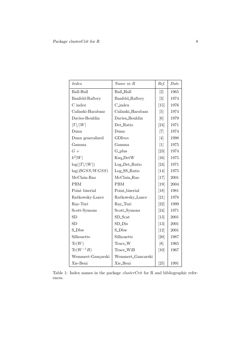
Package clusterCrit for R 8 Index Ball-Hall Name in R Ball Hall Banfeld-Raftery Banfeld Raftery C index C index Calinski-Harabasz Calinski Harabasz Davies-Bouldin |T|/|W| Dunn Dunn generalized Gamma G + k2|W| log(|T|/|W|) log(BGSS/W GSS) McClain-Rao PBM Davies Bouldin Det Ratio Dunn GDImn Gamma G plus Ksq DetW Log Det Ratio Log SS Ratio McClain Rao PBM Point biserial Point biserial Ratkowsky-Lance Ratkowsky Lance Ray-Turi Ray Turi Scott-Symons Scott Symons SD SD S Dbw Silhouette SD Scat SD Dis S Dbw Silhouette Tr(W ) Tr(W −1B) Wemmert-Gan¸carski Wemmert Gancarski Trace WiB Trace W Ref. Date [2] [3] [15] [5] [6] [24] [7] [4] [1] [23] [16] [24] [14] [17] [19] [18] [21] [22] [24] [13] [13] [12] [20] [8] [10] 1965 1974 1976 1974 1979 1971 1974 1998 1975 1974 1975 1971 1975 2001 2004 1981 1978 1999 1971 2001 2001 2001 1987 1965 1967 Xie-Beni Xie Beni [25] 1991 Table 1: Index names in the package clusterCrit for R and bibliographic refer- ences.

分享到：

赞收藏

资料库

聚类评估指标分析.pdf

相关推荐

人工智能

热门标签

最新资料