Foundations and Trends R in
Machine Learning
Vol. 4, No. 2 (2011) 107–194
c 2012 S. Shalev-Shwartz
DOI: 10.1561/2200000018
Online Learning and Online
Convex Optimization
By Shai Shalev-Shwartz
Contents
1 Introduction
1.1 Examples
1.2 A Gentle Start
1.3 Organization and Scope
1.4 Notation and Basic Definitions
2 Online Convex Optimization
2.1 Convexification
2.2 Follow-the-leader
2.3 Follow-the-Regularized-Leader
2.4 Online Gradient Descent: Linearization
of Convex Functions
2.5 Strongly Convex Regularizers
2.6 Online Mirror Descent
2.7 The Language of Duality
2.8 Bounds with Local Norms
2.9 Bibliographic Remarks
3 Online Classification
3.1 Finite Hypothesis Class and Experts Advice
3.2 Learnability and the Standard Optimal Algorithm
108
111
112
116
117
119
120
124
127
130
134
141
146
152
155
157
158
160
�
3.3 Perceptron and Winnow
3.4 Bibliographic Remarks
4 Limited Feedback (Bandits)
4.1 Online Mirror Descent with Estimated Gradients
4.2 The Multi-armed Bandit Problem
4.3 Gradient Descent Without a Gradient
4.4 Bibliographic Remarks
5 Online-to-Batch Conversions
5.1 Bibliographic Remarks
Acknowledgments
References
168
175
177
178
179
182
185
186
190
191
192
�
Foundations and Trends R in
Machine Learning
Vol. 4, No. 2 (2011) 107–194
c 2012 S. Shalev-Shwartz
DOI: 10.1561/2200000018
Online Learning and Online
Convex Optimization
Shai Shalev-Shwartz
Benin School of Computer Science and Engineering, The Hebrew University
of Jerusalem, Israel, shais@cs.huji.ac.il
Abstract
Online learning is a well established learning paradigm which has both
theoretical and practical appeals. The goal of online learning is to
make a sequence of accurate predictions given knowledge of the cor-
rect answer to previous prediction tasks and possibly additional avail-
able information. Online learning has been studied in several research
fields including game theory, information theory, and machine learning.
It also became of great interest to practitioners due the recent emer-
gence of large scale applications such as online advertisement placement
and online web ranking. In this survey we provide a modern overview
of online learning. Our goal is to give the reader a sense of some of
the interesting ideas and in particular to underscore the centrality of
convexity in deriving efficient online learning algorithms. We do not
mean to be comprehensive but rather to give a high-level, rigorous yet
easy to follow, survey.
�
1
Introduction
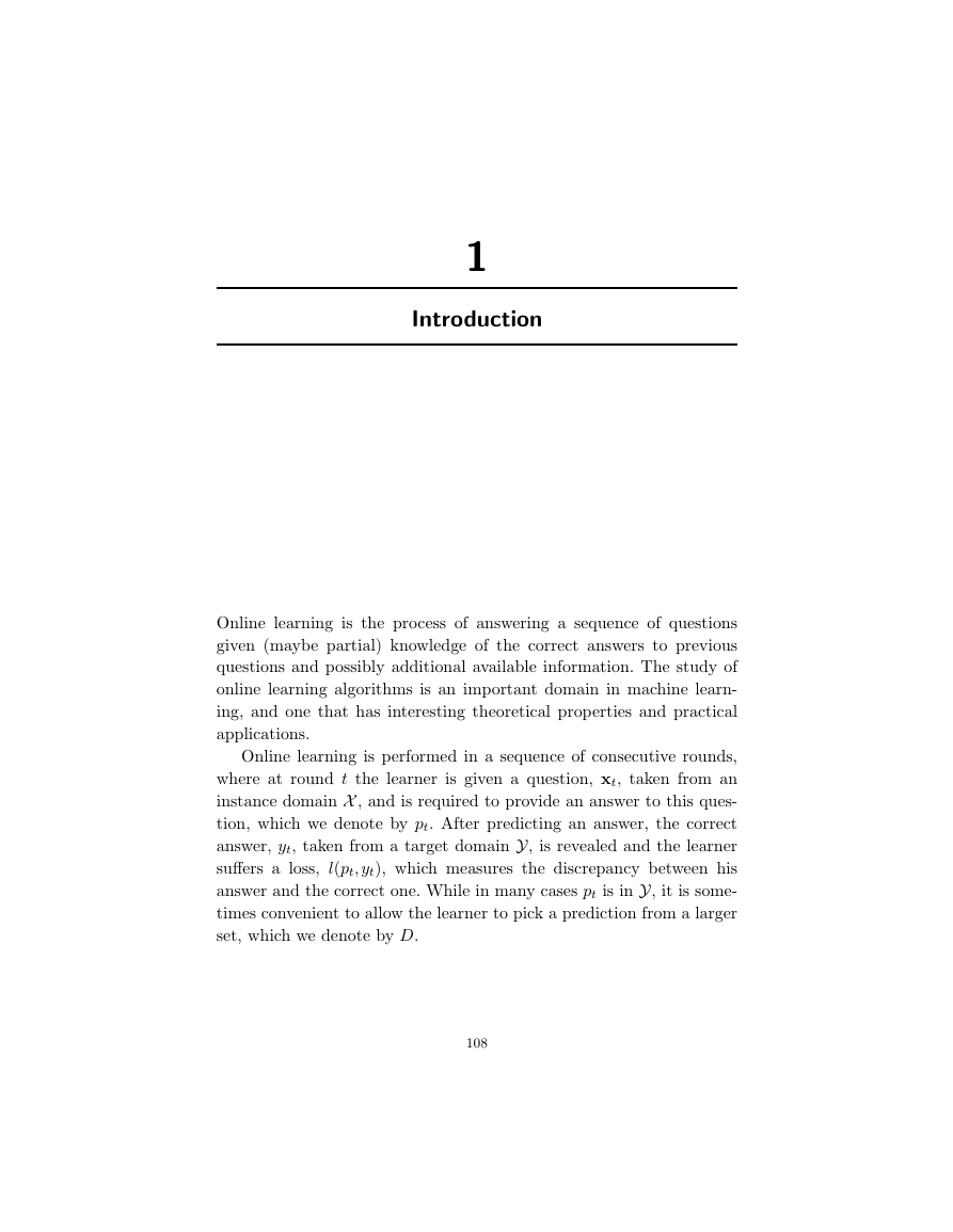
Online learning is the process of answering a sequence of questions
given (maybe partial) knowledge of the correct answers to previous
questions and possibly additional available information. The study of
online learning algorithms is an important domain in machine learn-
ing, and one that has interesting theoretical properties and practical
applications.
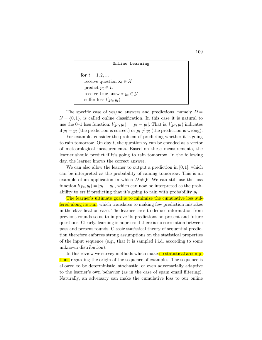
Online learning is performed in a sequence of consecutive rounds,
where at round t the learner is given a question, xt, taken from an
instance domain X , and is required to provide an answer to this ques-
tion, which we denote by pt. After predicting an answer, the correct
answer, yt, taken from a target domain Y, is revealed and the learner
suffers a loss, l(pt, yt), which measures the discrepancy between his
answer and the correct one. While in many cases pt is in Y, it is some-
times convenient to allow the learner to pick a prediction from a larger
set, which we denote by D.
108
�
109
Online Learning
for t = 1,2, . . .
receive question xt ∈ X
predict pt ∈ D
receive true answer yt ∈ Y
suffer loss l(pt, yt)
The specific case of yes/no answers and predictions, namely D =
Y = {0,1}, is called online classification. In this case it is natural to
use the 0–1 loss function: l(pt, yt) = |pt − yt|. That is, l(pt, yt) indicates
if pt = yt (the prediction is correct) or pt = yt (the prediction is wrong).
For example, consider the problem of predicting whether it is going
to rain tomorrow. On day t, the question xt can be encoded as a vector
of meteorological measurements. Based on these measurements, the
learner should predict if it’s going to rain tomorrow. In the following
day, the learner knows the correct answer.
We can also allow the learner to output a prediction in [0,1], which
can be interpreted as the probability of raining tomorrow. This is an
example of an application in which D = Y. We can still use the loss
function l(pt, yt) = |pt − yt|, which can now be interpreted as the prob-
ability to err if predicting that it’s going to rain with probability pt.
The learner’s ultimate goal is to minimize the cumulative loss suf-
fered along its run, which translates to making few prediction mistakes
in the classification case. The learner tries to deduce information from
previous rounds so as to improve its predictions on present and future
questions. Clearly, learning is hopeless if there is no correlation between
past and present rounds. Classic statistical theory of sequential predic-
tion therefore enforces strong assumptions on the statistical properties
of the input sequence (e.g., that it is sampled i.i.d. according to some
unknown distribution).
In this review we survey methods which make no statistical assump-
tions regarding the origin of the sequence of examples. The sequence is
allowed to be deterministic, stochastic, or even adversarially adaptive
to the learner’s own behavior (as in the case of spam email filtering).
Naturally, an adversary can make the cumulative loss to our online
�
110
Introduction
learning algorithm arbitrarily large. For example, the adversary can ask
the same question on each online round, wait for the learner’s answer,
and provide the opposite answer as the correct answer. To make non-
trivial statements we must further restrict the problem. We consider
two natural restrictions.
The first restriction is especially suited to the case of online classi-
fication. We assume that all the answers are generated by some target
mapping, h : X → Y. Furthermore, h is taken from a fixed set, called
a hypothesis class and denoted by H, which is known to the learner.
With this restriction on the sequence, which we call the realizable case,
the learner should make as few mistakes as possible, assuming that
both h and the sequence of questions can be chosen by an adversary.
For an online learning algorithm, A, we denote by MA(H) the max-
imal number of mistakes A might make on a sequence of examples
which is labeled by some h ∈ H. We emphasize again that both h
and the sequence of questions can be chosen by an adversary. A bound
on MA(H) is called a mistake-bound and we will study how to design
algorithms for which MA(H) is minimal.
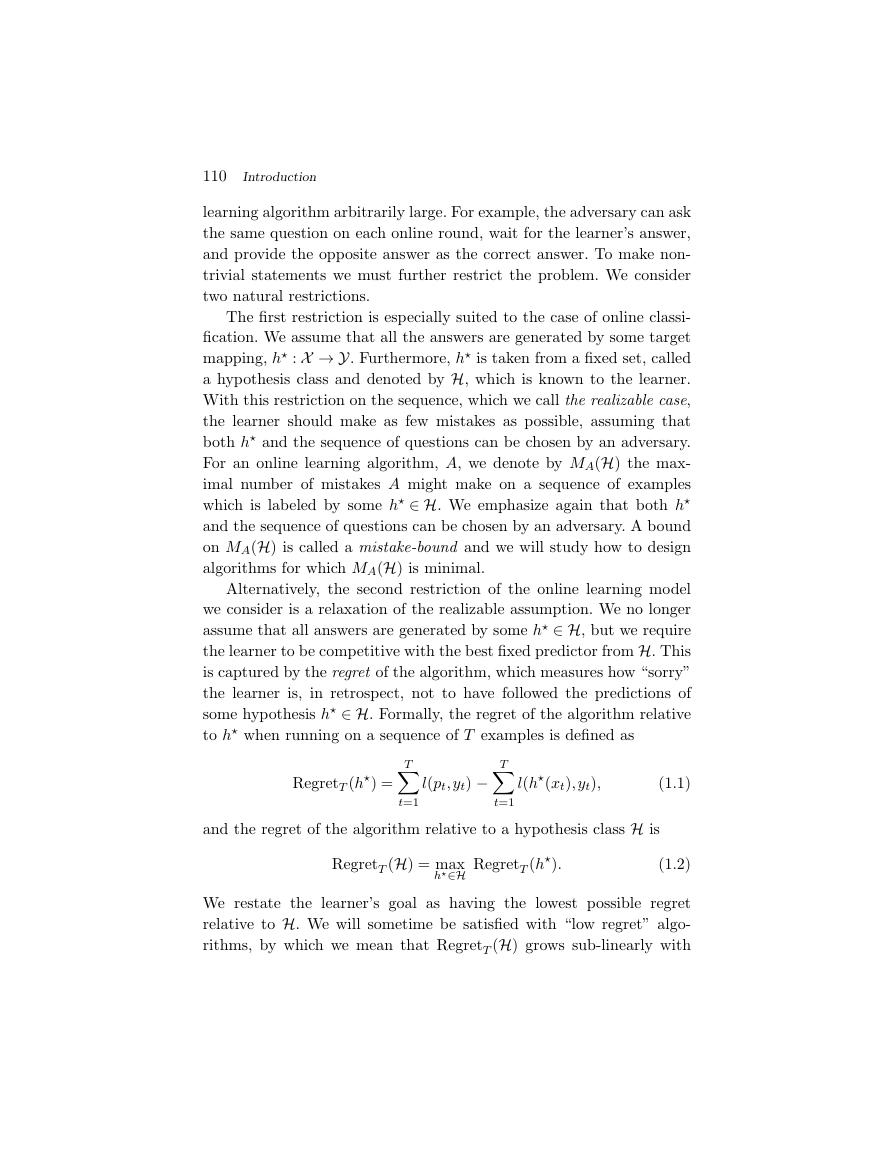
Alternatively, the second restriction of the online learning model
we consider is a relaxation of the realizable assumption. We no longer
assume that all answers are generated by some h ∈ H, but we require
the learner to be competitive with the best fixed predictor from H. This
is captured by the regret of the algorithm, which measures how “sorry”
the learner is, in retrospect, not to have followed the predictions of
some hypothesis h ∈ H. Formally, the regret of the algorithm relative
to h when running on a sequence of T examples is defined as
T
t=1
l(pt, yt) − T
t=1
RegretT (h) =
l(h(xt), yt),
(1.1)
and the regret of the algorithm relative to a hypothesis class H is
RegretT (H) = max
h∈H RegretT (h).
(1.2)
We restate the learner’s goal as having the lowest possible regret
relative to H. We will sometime be satisfied with “low regret” algo-
rithms, by which we mean that RegretT (H) grows sub-linearly with
�
the number of rounds, T , which implies that the difference between the
average loss of the learner and the average loss of the best hypothesis
in H tends to zero as T goes to infinity.
1.1 Examples
111
1.1 Examples
We already mentioned the problem of online classification. To make the
discussion more concrete, we list several additional online prediction
problems and possible hypothesis classes.
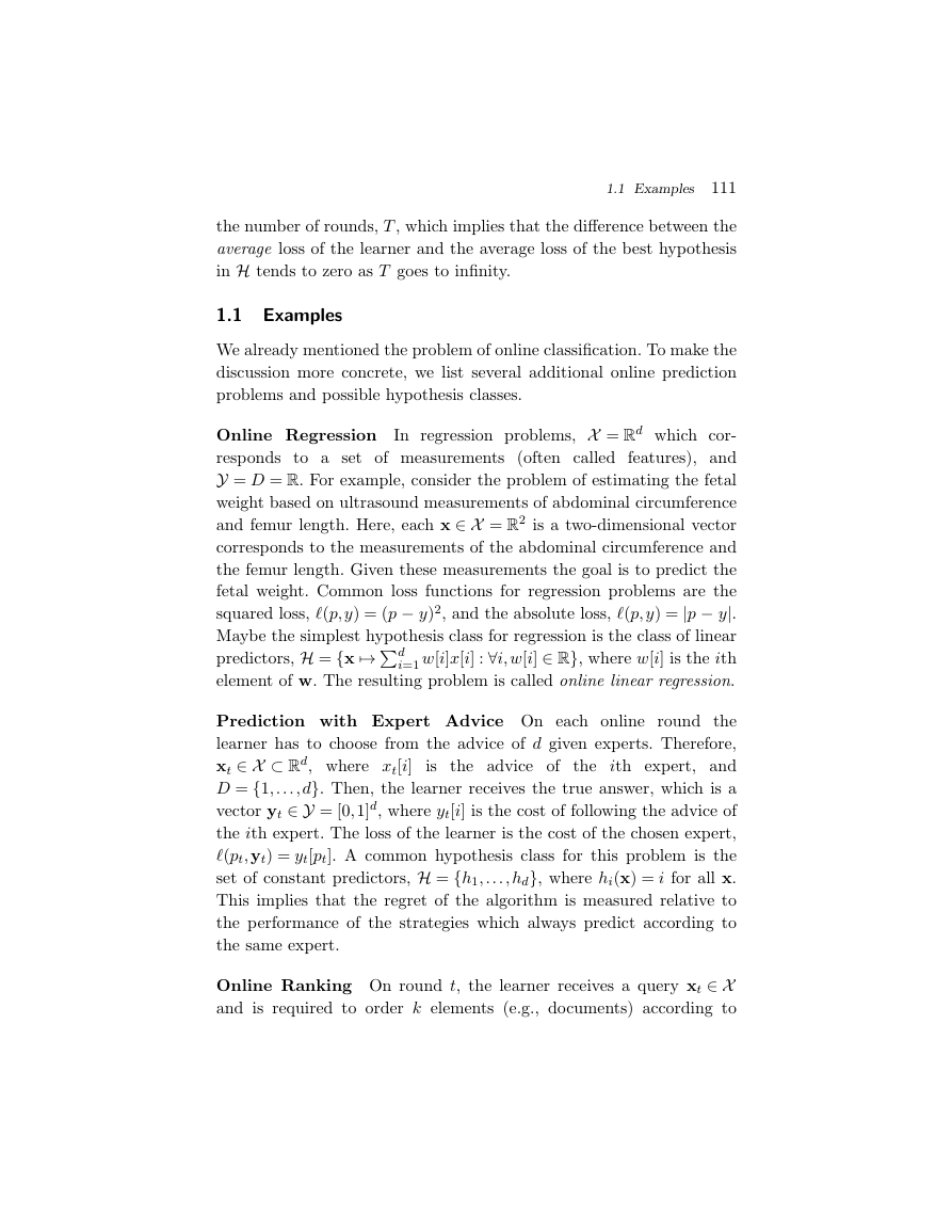
Online Regression In regression problems, X = Rd which cor-
responds to a set of measurements (often called features), and
Y = D = R. For example, consider the problem of estimating the fetal
weight based on ultrasound measurements of abdominal circumference
and femur length. Here, each x ∈ X = R2 is a two-dimensional vector
corresponds to the measurements of the abdominal circumference and
the femur length. Given these measurements the goal is to predict the
fetal weight. Common loss functions for regression problems are the
squared loss, (p, y) = (p − y)2, and the absolute loss, (p, y) = |p − y|.
Maybe the simplest hypothesis class for regression is the class of linear
i=1 w[i]x[i] : ∀i, w[i] ∈ R}, where w[i] is the ith
element of w. The resulting problem is called online linear regression.
predictors, H = {x →
d
Prediction with Expert Advice On each online round the
learner has to choose from the advice of d given experts. Therefore,
xt ∈ X ⊂ Rd, where xt[i]
is the advice of the ith expert, and
D = {1, . . . , d}. Then, the learner receives the true answer, which is a
vector yt ∈ Y = [0,1]d, where yt[i] is the cost of following the advice of
the ith expert. The loss of the learner is the cost of the chosen expert,
(pt,yt) = yt[pt]. A common hypothesis class for this problem is the
set of constant predictors, H = {h1, . . . , hd}, where hi(x) = i for all x.
This implies that the regret of the algorithm is measured relative to
the performance of the strategies which always predict according to
the same expert.
Online Ranking On round t, the learner receives a query xt ∈ X
and is required to order k elements (e.g., documents) according to
�
112
Introduction
their relevance to the query. That is, D is the set of all permuta-
tions of {1, . . . , k}. Then, the learner receives the true answer yt ∈ Y =
{1, . . . , k}, which corresponds to the document which best matches the
query. In web applications, this is the document that the user clicked
on. The loss, (pt, yt), is the position of yt in the ranked list pt.
1.2 A Gentle Start
We start with studying online classification problem, in which Y = D =
{0,1}, and (p, y) = |p − y| is the 0–1 loss. That is, on each round, the
learner receives xt ∈ X and is required to predict pt ∈ {0,1}. Then, it
receives yt ∈ {0,1} and pays the loss |pt − yt|. We make the following
simplifying assumption:
• Finite Hypothesis Class: We assume that |H| < ∞.
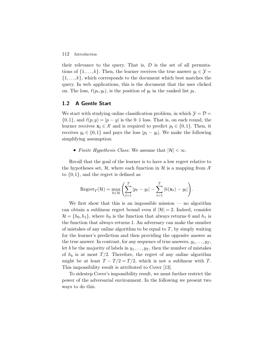
Recall that the goal of the learner is to have a low regret relative to
the hypotheses set, H, where each function in H is a mapping from X
to {0,1}, and the regret is defined as
T
RegretT (H) = max
h∈H
|pt − yt| − T
t=1
t=1
|h(xt) − yt|
.
We first show that this is an impossible mission — no algorithm
can obtain a sublinear regret bound even if |H| = 2. Indeed, consider
H = {h0, h1}, where h0 is the function that always returns 0 and h1 is
the function that always returns 1. An adversary can make the number
of mistakes of any online algorithm to be equal to T , by simply waiting
for the learner’s prediction and then providing the opposite answer as
the true answer. In contrast, for any sequence of true answers, y1, . . . , yT ,
let b be the majority of labels in y1, . . . , yT , then the number of mistakes
of hb is at most T /2. Therefore, the regret of any online algorithm
might be at least T − T /2 = T /2, which is not a sublinear with T .
This impossibility result is attributed to Cover [13].
To sidestep Cover’s impossibility result, we must further restrict the
power of the adversarial environment. In the following we present two
ways to do this.
�


 2023年江西萍乡中考道德与法治真题及答案.doc
 2012年重庆南川中考生物真题及答案.doc
 2013年江西师范大学地理学综合及文艺理论基础考研真题.doc
 2020年四川甘孜小升初语文真题及答案I卷.doc
 2020年注册岩土工程师专业基础考试真题及答案.doc
 2023-2024学年福建省厦门市九年级上学期数学月考试题及答案.doc
 2021-2022学年辽宁省沈阳市大东区九年级上学期语文期末试题及答案.doc
 2022-2023学年北京东城区初三第一学期物理期末试卷及答案.doc
 2018上半年江西教师资格初中地理学科知识与教学能力真题及答案.doc
 2012年河北国家公务员申论考试真题及答案-省级.doc
 2020-2021学年江苏省扬州市江都区邵樊片九年级上学期数学第一次质量检测试题及答案.doc
 2022下半年黑龙江教师资格证中学综合素质真题及答案.doc