Machine Learning, 54, 45–66, 2004
c 2004 Kluwer Academic Publishers. Manufactured in The Netherlands.
Support Vector Data Description
DAVID M.J. TAX
ROBERT P.W. DUIN
Pattern Recognition Group, Faculty of Applied Sciences, Delft University of Technology, Lorentzweg 1,
2628 CJ Delft, The Netherlands
davidt@first.fhg.de
r.p.w.duin@tnw.tudelft.nl
Editor: Douglas Fisher
Abstract. Data domain description concerns the characterization of a data set. A good description covers all
target data but includes no superfluous space. The boundary of a dataset can be used to detect novel data or outliers.
We will present the Support Vector Data Description (SVDD) which is inspired by the Support Vector Classifier.
It obtains a spherically shaped boundary around a dataset and analogous to the Support Vector Classifier it can be
made flexible by using other kernel functions. The method is made robust against outliers in the training set and is
capable of tightening the description by using negative examples. We show characteristics of the Support Vector
Data Descriptions using artificial and real data.
Keywords: outlier detection, novelty detection, one-class classification, support vector classifier, support vector
data description
1.
Introduction
Much effort has been expended to solve classification and regression tasks. In these problems
a mapping between objects represented by a feature vector and outputs (a class label or real
valued outputs) is inferred on the basis of a set of training examples. In practice, another type
of problem is of interest too: the problem of data description or One-Class Classification
(Moya, Koch, & Hostetler, 1993). Here the problem is to make a description of a training
set of objects and to detect which (new) objects resemble this training set.
Obviously data description can be used for outlier detection—to detect uncharacteristic
objects from a data set. Often these outliers in the data show an exceptionally large or small
feature value in comparison with other training objects. In general, trained classifiers or
regressors only provide reliable estimates for input data close to the training set. Extrapola-
tions to unknown and remote regions in feature space are very uncertain (Roberts & Penny,
1996). Neural networks, for instance, can be trained to estimate posterior probabilities
(Richard & Lippmann, 1991; Bishop, 1995; Ripley, 1996) and tend to give high confidence
outputs for objects which are remote from the training set. In these cases outlier detection
should be used first to detect and reject outliers to avoid unfounded confident classifications.
Secondly, data description can be used for a classification problem where one of the
classes is sampled very well, while the other class is severely undersampled. An example is
a machine monitoring system in which the current condition of a machine is examined. An
alarm is raised when the machine shows a problem. Measurements on the normal working
conditions of a machine are very cheap and easy to obtain. Measurements of outliers, on
�
46
D.M.J. TAX AND R.P.W. DUIN
the other hand, would require the destruction of the machine in all possible ways. It is very
expensive, if not impossible, to generate all faulty situations (Japkowicz, Myers, & Gluck,
1995). Only a method which uses mainly the target data, and does not require representative
outlier data, can solve this monitoring problem.
The last possible use of outlier detection is the comparison of two data sets. Assume a
classifier has been trained (by a long and difficult optimization) on some (possibly expensive)
data. When a similar problem has to be solved, the new data set can be compared with the
old training set. In case of incomparable data, the training of a new classifier will be needed.
In many one-class classification problems an extra complication occurs, namely that it
is beforehand not clear what the specific distribution of the data will be in practice. The
operator of the machine can easily run the machine in different, but legal modes, covering the
complete operational area of the machine. Although it defines the normal working area, the
distribution over this area is not to be trusted. In practice the machine may stay much longer
in one mode than in another, and this mode might have been sampled sparsely during the
training phase. A data description for this type of data should therefore model the boundary
of the normal class, instead of modeling the complete density distribution.
Several solutions for solving the data description problem have been proposed. Most
often the methods focus on outlier detection. Conceptually the simplest solution for outlier
detection is to generate outlier data around the target set. An ordinary classifier is then
trained to distinguish between the target data and outliers (Roberts et al., 1994). Koch
et al. (1995) used ART-2A and a Multi-Layered Perceptron for the detection of (partially
obscured) objects in an automatic target recognition system. Unfortunately this method
requires the availability of a set of near-target objects (possibly artificial) belonging to the
outlier class. The methods scale very poorly in high dimensional problems, especially when
the near-target data has to be created and is not readily available.
In classification or regression problems a more advanced Bayesian approach can be used
for detecting outliers (Bishop, 1995; MacKay, 1992; Roberts & Penny, 1996). Instead of
using the most probable weight configuration of a classifier (or regressor) to compute the
output, the output is weighted by the probability that the weight configuration is correct
given the data. This method can then provide an estimate of the probability for a certain
object given the model family. Low probabilities will then indicate a possible outlier. The
classifier outputs are moderated automatically for objects remote from the training domain.
These methods are not optimized for outlier detection though; they require a classification
(or regression) task to be solved and can be computationally expensive.
Most often the task of data description is solved by estimating a probability density of the
target data (Barnett & Lewis, 1978). For instance in Bishop (1994) and Tarassenko, Hayton,
and Brady (1995) the density is estimated by a Parzen density estimator, whereas in Parra,
Deco, and Miesbach (1996) one Gaussian distribution is used. In (Ritter & Gallegos, 1997)
not only the target density is estimated, but also the outlier density. The first drawback is that
in general (in higher dimensional feature spaces) a large number of samples is required. The
second drawback is that they will not be very resistant to training data which only defines
the area of the target data, and which does not represent the complete density distribution. It
will mainly focus on modeling the high density areas, and reject low density areas, although
they may define legal target data.
�
SUPPORT VECTOR DATA DESCRIPTION
47
Vapnik argued that in order to solve a problem, one should not try to solve a more
general problem as an intermediate step (Vapnik, 1998). The estimation of the complete
density instead of computing the boundary around a data set might require too much data
and could result in bad descriptions. An attempt to train just the boundaries of a data set
is made in Moya and Hush (1996) and Moya, Koch, and Hostetler (1993). Here neural
networks are trained with extra constraints to give closed boundaries. Unfortunately this
method inherits the weak points in neural network training, i.e. the choice of the size of
the network, weight initialization, the stopping criterion, etc. Rosen (1965) made a data
description as a by-product of a classification problem. He shows how the classification
problem can be formulated as a convex programming problem. When the classification
problem is not linearly separable, an ellipsoidal separation can be applied, where one of the
classes is enclosed by an ellipsoid of minimum size. We will use a similar method for the
one-class classification problem.
Finally Sch¨olkopf et al. used an hyperplane (Sch¨olkopf et al., 1999b) to separate the
target objects from the origin with maximal margin. This formulation is comparable with
the Support Vector Classifier by Vapnik (1998) and it is possible to define implicit mappings
to obtain more flexible descriptions.
In this paper we discuss a method which obtains a spherically shaped boundary around the
complete target set with the same flexibility. To minimize the chance of accepting outliers,
the volume of this description is minimized. We will show how the outlier sensitivity can
be controlled by changing the ball-shaped boundary into a more flexible boundary and how
example outliers can be included into the training procedure (when they are available) to
find a more efficient description.
In Section 2 we present the basic theory, which is presented in part in Tax and Duin
(1999). The normal data description, and also the description using negative examples will
be explained and we will compare the method with the hyperplane approach in Sch¨olkopf
et al. (1999b). In Section 3 some basic characteristics of this data description will be shown,
and in Section 4 the method will be applied to a real life problem and compared with some
other density estimation methods. Section 5 contains some conclusions.
2. Theory
To begin, we fix some notation. We assume vectors x are column vectors and x2 = x · x.
We have a training set {xi}, i = 1, . . . , N for which we want to obtain a description. We
further assume that the data shows variances in all feature directions.
2.1. Normal data description
To start with the normal data description, we define a model which gives a closed boundary
around the data: an hypersphere. The sphere is characterized by center a and radius R > 0.
We minimize the volume of the sphere by minimizing R2, and demand that the sphere
contains all training objects xi . This is identical to the approach which is used in Sch¨olkopf,
Burges, and Vapnik (1995) to estimate the VC-dimension of a classifier (which is bounded
by the diameter of the smallest sphere enclosing the data). At the end of this section we will
�
48
D.M.J. TAX AND R.P.W. DUIN
show that this approach gives solutions similar to the hyperplane approach of Sch¨olkopf
et al. (1999b).
Analogous to the Support Vector Classifier (Vapnik, 1998) we define the error function
to minimize:
F(R, a) = R2
with the constraints:
xi − a2 ≤ R2, ∀i
(1)
(2)
To allow the possibility of outliers in the training set, the distance from xi to the center a
should not be strictly smaller than R2, but larger distances should be penalized. Therefore
we introduce slack variables ξi ≥ 0 and the minimization problem changes into:
F(R, a) = R2 + C
ξi
i
with constraints that almost all objects are within the sphere:
xi − a2 ≤ R2 + ξi ,
ξi ≥ 0 ∀i
(3)
(4)
The parameter C controls the trade-off between the volume and the errors.
Constraints (4) can be incorporated into Eq. (3) by using Lagrange multipliers:
L(R, a, αi , γi , ξi ) = R2 + C
ξi
i
αi{R2 + ξi − (xi2 − 2a · xi + a2)} −
−
i
i
γi ξi
(5)
with the Lagrange multipliers αi ≥ 0 and γi ≥ 0. L should be minimized with respect to
R, a, ξi and maximized with respect to αi and γi .
Setting partial derivatives to zero gives the constraints:
=
αi xi
(6)
(7)
i
a =
αi = 1
αi xi
i
αi
i
i
C − αi − γi = 0
= 0 :
= 0 :
= 0 :
∂ L
∂ R
∂ L
∂a
∂ L
∂ξi
(8)
From the last equation αi = C − γi and because αi ≥ 0, γi ≥ 0, Lagrange multipliers γi
can be removed when we demand that
0 ≤ αi ≤ C
(9)
�
SUPPORT VECTOR DATA DESCRIPTION
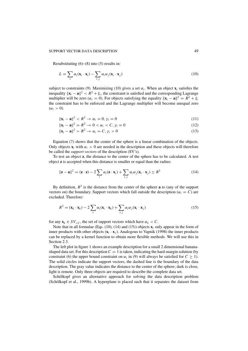
Resubstituting (6)–(8) into (5) results in:
αi α j (xi · x j )
αi (xi · xi ) −
L =
49
(10)
i
i, j
subject to constraints (9). Maximizing (10) gives a set αi . When an object xi satisfies the
inequality xi − a2 < R2 + ξi , the constraint is satisfied and the corresponding Lagrange
multiplier will be zero (αi = 0). For objects satisfying the equality xi − a2 = R2 + ξi
the constraint has to be enforced and the Lagrange multiplier will become unequal zero
(αi > 0).
xi − a2 < R2 → αi = 0, γi = 0
xi − a2 = R2 → 0 < αi < C, γi = 0
xi − a2 > R2 → αi = C, γi > 0
(11)
(12)
(13)
Equation (7) shows that the center of the sphere is a linear combination of the objects.
Only objects xi with αi > 0 are needed in the description and these objects will therefore
be called the support vectors of the description (SV’s).
To test an object z, the distance to the center of the sphere has to be calculated. A test
object z is accepted when this distance is smaller or equal than the radius:
z − a2 = (z · z) − 2
αi (z · xi ) +
αi α j (xi · x j ) ≤ R2
(14)
i
i, j
By definition, R2 is the distance from the center of the sphere a to (any of the support
vectors on) the boundary. Support vectors which fall outside the description (αi = C) are
excluded. Therefore:
R2 = (xk · xk) − 2
αi (xi · xk) +
αi α j (xi · x j )
(15)
i
i, j
for any xk ∈ SV
50
D.M.J. TAX AND R.P.W. DUIN
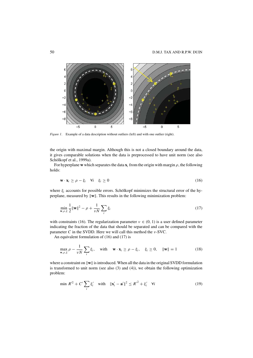
Figure 1. Example of a data description without outliers (left) and with one outlier (right).
the origin with maximal margin. Although this is not a closed boundary around the data,
it gives comparable solutions when the data is preprocessed to have unit norm (see also
Sch¨olkopf et al., 1999a).
For hyperplane w which separates the data xi from the origin with margin ρ, the following
holds:
w · xi ≥ ρ − ξi
∀i
ξi ≥ 0
(16)
where ξi accounts for possible errors. Sch¨olkopf minimizes the structural error of the hy-
perplane, measured by w. This results in the following minimization problem:
1
2
w2 − ρ + 1
ν N
min
w,ρ,ξ
ξi
i
(17)
with constraints (16). The regularization parameter ν ∈ (0, 1) is a user defined parameter
indicating the fraction of the data that should be separated and can be compared with the
parameter C in the SVDD. Here we will call this method the ν-SVC.
An equivalent formulation of (16) and (17) is
ξi , with w · xi ≥ ρ − ξi ,
ξi ≥ 0,
w = 1
(18)
ρ − 1
ν N
max
w,ρ,ξ
i
i
where a constraint onw is introduced. When all the data in the original SVDD formulation
is transformed to unit norm (see also (3) and (4)), we obtain the following optimization
problem:
min R
2 + C
ξ
i with
x
i
− a
2 ≤ R
2 + ξ
i
∀i
(19)
�
SUPPORT VECTOR DATA DESCRIPTION
where x
and a
max−R
ξ
i with
are normalized vectors. Rewriting gives:
2 − C
i ) ≥ 2 − R
, ξi = ξ
= C
· x
2(a
2, 1
ν N
i
2 − ξ
i
We define w = 2a, ρ = 2 − R
problem is obtained:
max −2 + ρ − 1
ν N
i
i and the following optimization
ξi with w · xi ≥ ρ − ξi ,
ξi ≥ 0,
w = 2
(21)
which is a comparable solution to Eq. (18). It differs in the constraint on the norm of w
and in an offset of 2 in the error function. For non-normalized data the solutions become
incomparable due to the difference in model of the description (hyperplane or hypersphere).
We will come back to the ν-SVC in Section 2.3 in the discussion on kernels.
2.2.
SVDD with negative examples
When negative examples (objects which should be rejected) are available, they can be
incorporated in the training to improve the description. In contrast with the training (target)
examples which should be within the sphere, the negative examples should be outside it.
This data description now differs from the normal Support Vector Classifier in the fact that
the SVDD always obtains a closed boundary around one of the classes (the target class).
The support vector classifier just distinguishes between two (or more) classes and cannot
detect outliers which do not belong to any of the classes.
In the following the target objects are enumerated by indices i, j and the negative examples
by l, m. For further convenience assume that target objects are labeled yi = 1 and outlier
objects are labeled yl = −1. Again we allow for errors in both the target and the outlier set
and introduce slack variables ξi and ξl:
51
(20)
(22)
(23)
F(R, a, ξi , ξl) = R2 + C1
ξi + C2
ξl
l
and the constraints
i
xi − a2 ≤ R2 + ξi , xl − a2 ≥ R2 − ξl ,
ξi ≥ 0, ξl ≥ 0 ∀i, l
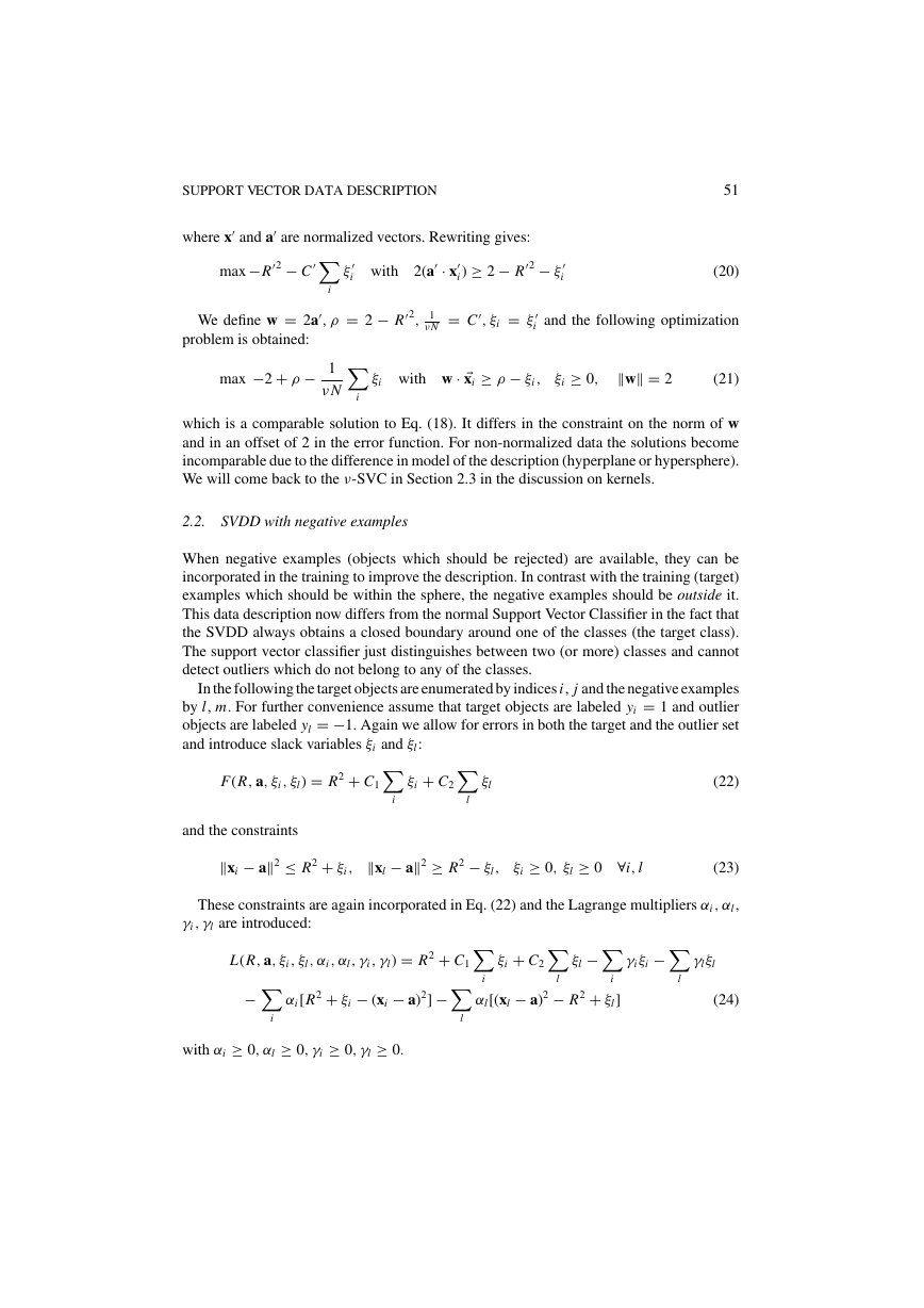
These constraints are again incorporated in Eq. (22) and the Lagrange multipliers αi , αl,
γi , γl are introduced:
L(R, a, ξi , ξl , αi , αl , γi , γl) = R2 + C1
−
αi [R2 + ξi − (xi − a)2] −
i
l
with αi ≥ 0, αl ≥ 0, γi ≥ 0, γl ≥ 0.
ξi + C2
ξl −
γi ξi −
i
l
i
αl[(xl − a)2 − R2 + ξl]
γl ξl
l
(24)
�
52
D.M.J. TAX AND R.P.W. DUIN
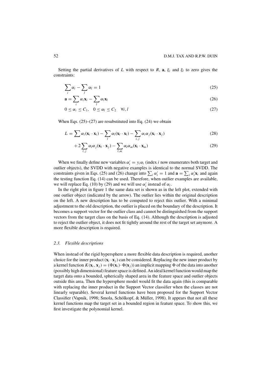
Setting the partial derivatives of L with respect to R, a, ξi and ξl to zero gives the
constraints:
αi −
i
l
αl = 1
αi xi −
a =
0 ≤ αi ≤ C1, 0 ≤ αl ≤ C2 ∀i, l
αlxl
i
l
When Eqs. (25)–(27) are resubstituted into Eq. (24) we obtain
L =
+ 2
αi (xi · xi ) −
l
αl α j (xl · x j ) −
αl(xl · xl) −
i, j
αl αm(xl · xm)
αi α j (xi · x j )
(25)
(26)
(27)
(28)
(29)
l, j
l,m
i
i
i
When we finally define new variables α
= yi αi (index i now enumerates both target and
outlier objects), the SVDD with negative examples is identical to the normal SVDD. The
α
i xi and again
constraints given in Eqs. (25) and (26) change into
the testing function Eq. (14) can be used. Therefore, when outlier examples are available,
we will replace Eq. (10) by (29) and we will use α
= 1 and a =
α
i instead of αi .
In the right plot in figure 1 the same data set is shown as in the left plot, extended with
one outlier object (indicated by the arrow). The outlier lies within the original description
on the left. A new description has to be computed to reject this outlier. With a minimal
adjustment to the old description, the outlier is placed on the boundary of the description. It
becomes a support vector for the outlier class and cannot be distinguished from the support
vectors from the target class on the basis of Eq. (14). Although the description is adjusted
to reject the outlier object, it does not fit tightly around the rest of the target set anymore. A
more flexible description is required.
i
2.3. Flexible descriptions
When instead of the rigid hypersphere a more flexible data description is required, another
choice for the inner product (xi · x j ) can be considered. Replacing the new inner product by
a kernel function K (xi , x j ) = (�(xi )· �(x j )) an implicit mapping � of the data into another
(possibly high dimensional) feature space is defined. An ideal kernel function would map the
target data onto a bounded, spherically shaped area in the feature space and outlier objects
outside this area. Then the hypersphere model would fit the data again (this is comparable
with replacing the inner product in the Support Vector classifier when the classes are not
linearly separable). Several kernel functions have been proposed for the Support Vector
Classifier (Vapnik, 1998; Smola, Sch¨olkopf, & M¨uller, 1998). It appears that not all these
kernel functions map the target set in a bounded region in feature space. To show this, we
first investigate the polynomial kernel.
�


 2023年江西萍乡中考道德与法治真题及答案.doc
 2012年重庆南川中考生物真题及答案.doc
 2013年江西师范大学地理学综合及文艺理论基础考研真题.doc
 2020年四川甘孜小升初语文真题及答案I卷.doc
 2020年注册岩土工程师专业基础考试真题及答案.doc
 2023-2024学年福建省厦门市九年级上学期数学月考试题及答案.doc
 2021-2022学年辽宁省沈阳市大东区九年级上学期语文期末试题及答案.doc
 2022-2023学年北京东城区初三第一学期物理期末试卷及答案.doc
 2018上半年江西教师资格初中地理学科知识与教学能力真题及答案.doc
 2012年河北国家公务员申论考试真题及答案-省级.doc
 2020-2021学年江苏省扬州市江都区邵樊片九年级上学期数学第一次质量检测试题及答案.doc
 2022下半年黑龙江教师资格证中学综合素质真题及答案.doc