CSRNet网络用于高度拥挤场景.pdf

发布时间：2022-06-19 发布人：admin 分类：说明书资料大小：8.73M 资料格式：pdf 举报版权申诉

7abed441-143f-48b3-b0cf-4e303c5bcd92.pdf-第1页.png

第1页 / 共16页

7abed441-143f-48b3-b0cf-4e303c5bcd92.pdf-第2页.png

第2页 / 共16页

7abed441-143f-48b3-b0cf-4e303c5bcd92.pdf-第3页.png

第3页 / 共16页

7abed441-143f-48b3-b0cf-4e303c5bcd92.pdf-第4页.png

第4页 / 共16页

7abed441-143f-48b3-b0cf-4e303c5bcd92.pdf-第5页.png

第5页 / 共16页

7abed441-143f-48b3-b0cf-4e303c5bcd92.pdf-第6页.png

第6页 / 共16页

7abed441-143f-48b3-b0cf-4e303c5bcd92.pdf-第7页.png

第7页 / 共16页

7abed441-143f-48b3-b0cf-4e303c5bcd92.pdf-第8页.png

第8页 / 共16页

文本预览

CSRNet: Dilated Convolutional Neural Networks for Understanding the Highly Congested Scenes Yuhong Li1,2, Xiaofan Zhang1, Deming Chen1 1University of Illinois at Urbana-Champaign 2Beijing University of Posts and Telecommunications {leeyh,xiaofan3,dchen}@illinois.edu 8 1 0 2 r p A 1 1 ] V C . s c [ 4 v 2 6 0 0 1 . 2 0 8 1 : v i X r a Abstract We propose a network for Congested Scene Recognition called CSRNet to provide a data-driven and deep learning method that can understand highly congested scenes and perform accurate count estimation as well as present high- quality density maps. The proposed CSRNet is composed of two major components: a convolutional neural network (CNN) as the front-end for 2D feature extraction and a di- lated CNN for the back-end, which uses dilated kernels to deliver larger reception ﬁelds and to replace pooling opera- tions. CSRNet is an easy-trained model because of its pure convolutional structure. We demonstrate CSRNet on four datasets (ShanghaiTech dataset, the UCF CC 50 dataset, the WorldEXPO’10 dataset, and the UCSD dataset) and we deliver the state-of-the-art performance. In the Shang- haiTech Part B dataset, CSRNet achieves 47.3% lower Mean Absolute Error (MAE) than the previous state-of-the- art method. We extend the targeted applications for count- ing other objects, such as the vehicle in TRANCOS dataset. Results show that CSRNet signiﬁcantly improves the output quality with 15.4% lower MAE than the previous state-of- the-art approach. 1. Introduction Growing number of network models have been devel- oped [1, 2, 3, 4, 5] to deliver promising solutions for crowd ﬂows monitoring, assembly controlling, and other security services. Current methods for congested scenes analysis are developed from simple crowd counting (which outputs the number of people in the targeted image) to density map pre- senting (which displays characteristics of crowd distribu- tion) [6]. 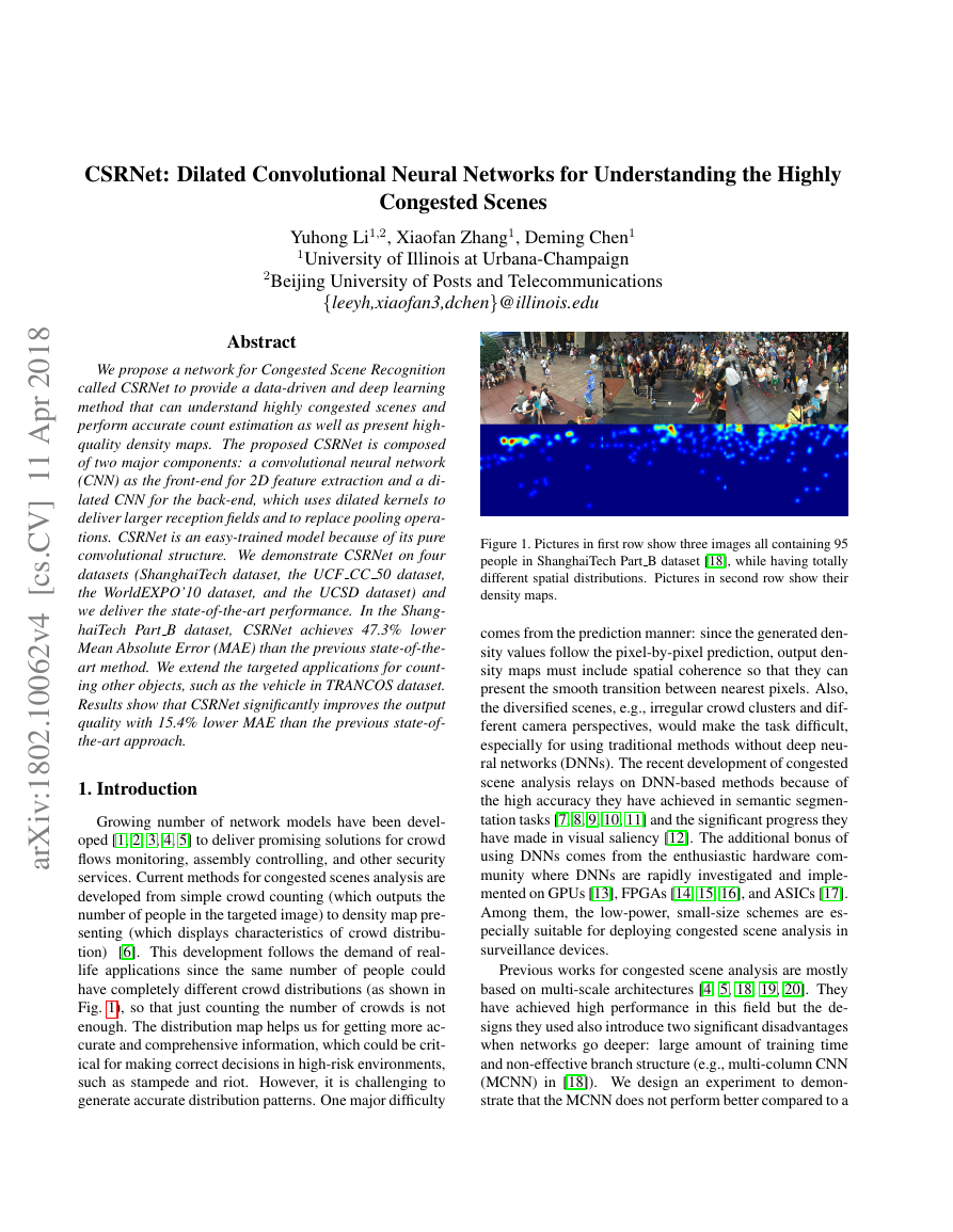This development follows the demand of real- life applications since the same number of people could have completely different crowd distributions (as shown in Fig. 1), so that just counting the number of crowds is not enough. The distribution map helps us for getting more ac- curate and comprehensive information, which could be crit- ical for making correct decisions in high-risk environments, such as stampede and riot. However, it is challenging to generate accurate distribution patterns. One major difﬁculty Figure 1. Pictures in ﬁrst row show three images all containing 95 people in ShanghaiTech Part B dataset [18], while having totally different spatial distributions. Pictures in second row show their density maps. comes from the prediction manner: since the generated den- sity values follow the pixel-by-pixel prediction, output den- sity maps must include spatial coherence so that they can present the smooth transition between nearest pixels. Also, the diversiﬁed scenes, e.g., irregular crowd clusters and dif- ferent camera perspectives, would make the task difﬁcult, especially for using traditional methods without deep neu- ral networks (DNNs). The recent development of congested scene analysis relays on DNN-based methods because of the high accuracy they have achieved in semantic segmen- tation tasks [7, 8, 9, 10, 11] and the signiﬁcant progress they have made in visual saliency [12]. The additional bonus of using DNNs comes from the enthusiastic hardware com- munity where DNNs are rapidly investigated and imple- mented on GPUs [13], FPGAs [14, 15, 16], and ASICs [17]. Among them, the low-power, small-size schemes are es- pecially suitable for deploying congested scene analysis in surveillance devices. Previous works for congested scene analysis are mostly based on multi-scale architectures [4, 5, 18, 19, 20]. They have achieved high performance in this ﬁeld but the de- signs they used also introduce two signiﬁcant disadvantages when networks go deeper: large amount of training time and non-effective branch structure (e.g., multi-column CNN (MCNN) in [18]). We design an experiment to demon- strate that the MCNN does not perform better compared to a

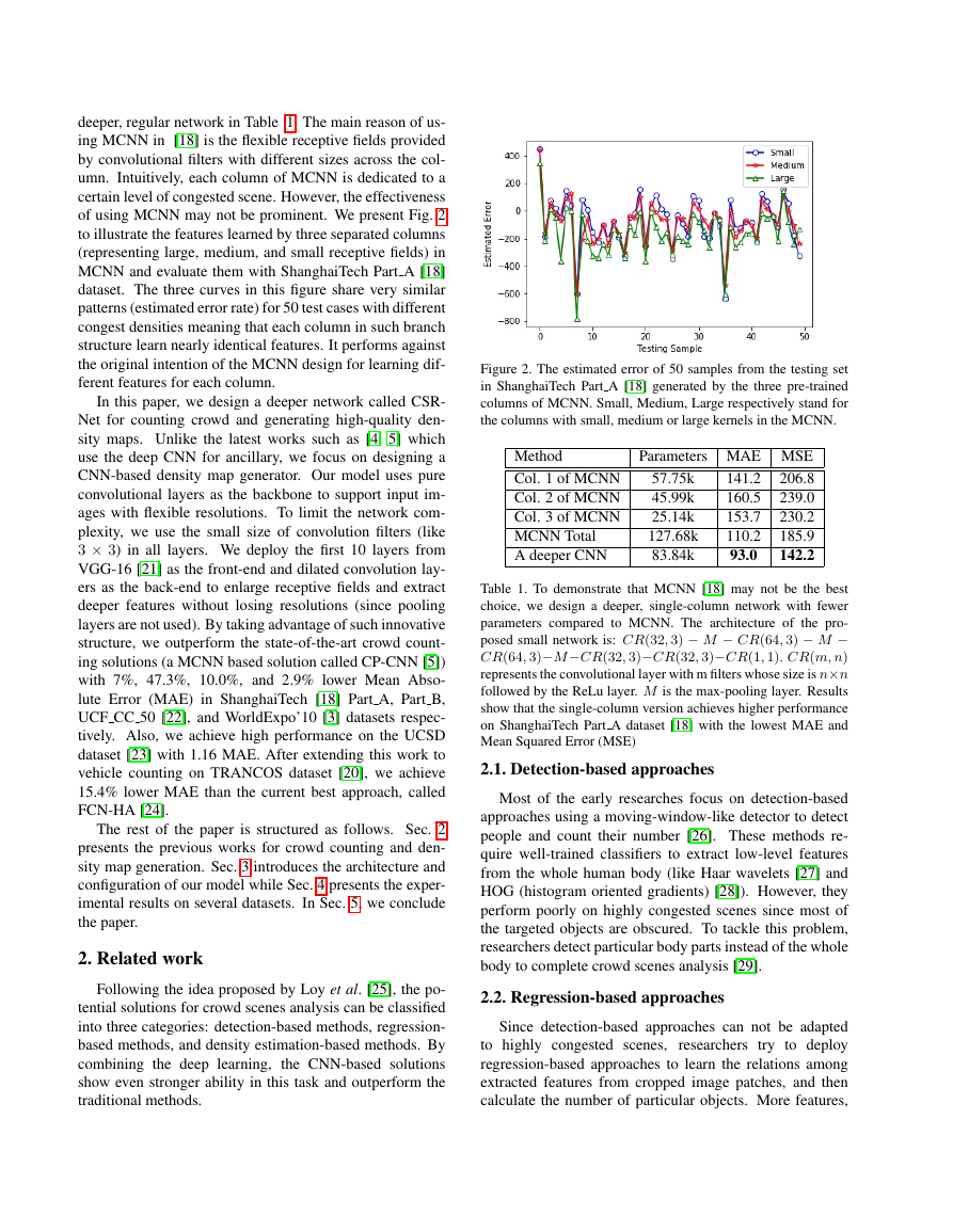
deeper, regular network in Table 1. The main reason of us- ing MCNN in [18] is the ﬂexible receptive ﬁelds provided by convolutional ﬁlters with different sizes across the col- umn. Intuitively, each column of MCNN is dedicated to a certain level of congested scene. However, the effectiveness of using MCNN may not be prominent. We present Fig. 2 to illustrate the features learned by three separated columns (representing large, medium, and small receptive ﬁelds) in MCNN and evaluate them with ShanghaiTech Part A [18] dataset. The three curves in this ﬁgure share very similar patterns (estimated error rate) for 50 test cases with different congest densities meaning that each column in such branch structure learn nearly identical features. It performs against the original intention of the MCNN design for learning dif- ferent features for each column. In this paper, we design a deeper network called CSR- Net for counting crowd and generating high-quality den- sity maps. Unlike the latest works such as [4, 5] which use the deep CNN for ancillary, we focus on designing a CNN-based density map generator. Our model uses pure convolutional layers as the backbone to support input im- ages with ﬂexible resolutions. To limit the network com- plexity, we use the small size of convolution ﬁlters (like 3 × 3) in all layers. We deploy the ﬁrst 10 layers from VGG-16 [21] as the front-end and dilated convolution lay- ers as the back-end to enlarge receptive ﬁelds and extract deeper features without losing resolutions (since pooling layers are not used). By taking advantage of such innovative structure, we outperform the state-of-the-art crowd count- ing solutions (a MCNN based solution called CP-CNN [5]) with 7%, 47.3%, 10.0%, and 2.9% lower Mean Abso- lute Error (MAE) in ShanghaiTech [18] Part A, Part B, UCF CC 50 [22], and WorldExpo’10 [3] datasets respec- tively. Also, we achieve high performance on the UCSD dataset [23] with 1.16 MAE. After extending this work to vehicle counting on TRANCOS dataset [20], we achieve 15.4% lower MAE than the current best approach, called FCN-HA [24]. The rest of the paper is structured as follows. Sec. 2 presents the previous works for crowd counting and den- sity map generation. Sec. 3 introduces the architecture and conﬁguration of our model while Sec. 4 presents the exper- imental results on several datasets. In Sec. 5, we conclude the paper. 2. Related work Following the idea proposed by Loy et al. [25], the po- tential solutions for crowd scenes analysis can be classiﬁed into three categories: detection-based methods, regression- based methods, and density estimation-based methods. By combining the deep learning, the CNN-based solutions show even stronger ability in this task and outperform the traditional methods. Figure 2. The estimated error of 50 samples from the testing set in ShanghaiTech Part A [18] generated by the three pre-trained columns of MCNN. Small, Medium, Large respectively stand for the columns with small, medium or large kernels in the MCNN. Method Col. 1 of MCNN Col. 2 of MCNN Col. 3 of MCNN MCNN Total A deeper CNN Parameters MAE MSE 206.8 239.0 230.2 185.9 142.2 57.75k 45.99k 25.14k 127.68k 83.84k 141.2 160.5 153.7 110.2 93.0 Table 1. To demonstrate that MCNN [18] may not be the best choice, we design a deeper, single-column network with fewer parameters compared to MCNN. The architecture of the pro- posed small network is: CR(32, 3) − M − CR(64, 3) − M − CR(64, 3)−M−CR(32, 3)−CR(32, 3)−CR(1, 1). CR(m, n) represents the convolutional layer with m ﬁlters whose size is n×n followed by the ReLu layer. M is the max-pooling layer. Results show that the single-column version achieves higher performance on ShanghaiTech Part A dataset [18] with the lowest MAE and Mean Squared Error (MSE) 2.1. Detection-based approaches Most of the early researches focus on detection-based approaches using a moving-window-like detector to detect people and count their number [26]. These methods re- quire well-trained classiﬁers to extract low-level features from the whole human body (like Haar wavelets [27] and HOG (histogram oriented gradients) [28]). However, they perform poorly on highly congested scenes since most of the targeted objects are obscured. To tackle this problem, researchers detect particular body parts instead of the whole body to complete crowd scenes analysis [29]. 2.2. Regression-based approaches Since detection-based approaches can not be adapted to highly congested scenes, researchers try to deploy regression-based approaches to learn the relations among extracted features from cropped image patches, and then calculate the number of particular objects. More features,

such as foreground and texture features, have been used for generating low-level information [30]. Following similar approaches, Idrees et al. [22] propose a model to extract features by employing Fourier analysis and SIFT (Scale- invariant feature transform) [31] interest-point based count- ing. 2.3. Density estimation-based approaches When executing the regression-based solution, one crit- ical feature, called saliency, is overlooked which causes in- accurate results in local regions. Lempitsky et al. [32] pro- pose a method to solve this problem by learning a linear mapping between features in the local region and its object density maps. It integrates the information of saliency dur- ing the learning process. Since the ideal linear mapping is hard to obtain, Pham et al. [33] use random forest regression to learn a non-linear mapping instead of the linear one. 2.4. CNN-based approaches Literature also focuses on the CNN-based approaches to predict the density map because of its success in clas- siﬁcation and recognition [34, 21, 35]. In the work pre- sented by Walach and Wolf [36], a method is demonstrated with selective sampling and layered boosting. Instead of using patch-based training, Shang et al. [37] try an end-to- end regression method using CNNs which takes the entire image as input and directly outputs the ﬁnal crowd count. Boominathan et al. [19] present the ﬁrst work purely us- ing convolutional networks and dual-column architecture for generating density map. Marsden et al. [38] explore single-column fully convolutional networks while Sindagi et al. [39] propose a CNN which uses the high-level prior in- formation to boost the density prediction performance. An improved structure is proposed by Zhang et al. [18] who introduce a multi-column based architecture (MCNN) for crowd counting. Similar idea is shown in Onoro and Sas- tre [20] where a scale-aware, multi-column counting model called Hydra CNN is presented for object density estima- tion. It is clear that the CNN-based solutions outperform the previous works mentioned in Sec. 2.1 to 2.3. 2.5. Limitations of the state-of-the-art approaches Most recently, Sam et al. [4] propose the Switch-CNN using a density level classiﬁer to choose different regres- sors for particular input patches. Sindagi et al. [5] present a Contextual Pyramid CNN, which uses CNN networks to estimate context at various levels for achieving lower count error and better quality density maps. These two solutions achieve the state-of-the-art performance, and both of them used multi-column based architecture (MCNN) and den- sity level classiﬁer. However, we observe several disad- vantages in these approaches: (1) Multi-column CNNs are hard to train according to the training method described in work [18]. Such bloated network structure requires more time to train. (2) Multi-column CNNs introduce redundant structure as we mentioned in Sec. 1. Different columns seem to perform similarly without obvious differences. (3) Both solutions require density level classiﬁer before send- ing pictures in the MCNN. However, the granularity of den- sity level is hard to deﬁne in real-time congested scene anal- ysis since the number of objects keeps changing with a large range. Also, using a ﬁne-grained classiﬁer means more columns need to be implemented which makes the design more complicated and causes more redundancy. (4) These works spend a large portion of parameters for density level classiﬁcation to label the input regions instead of allocating parameters to the ﬁnal density map generation. Since the branch structure in MCNN is not efﬁcient, the lack of pa- rameters for generating density map lowers the ﬁnal accu- racy. Taking all above disadvantages into consideration, we propose a novel approach to concentrate on encoding the deeper features in congested scenes and generating high- quality density map. 3. Proposed Solution The fundamental idea of the proposed design is to de- ploy a deeper CNN for capturing high-level features with larger receptive ﬁelds and generating high-quality density maps without brutally expanding network complexity. In this section, we ﬁrst introduce the architecture we proposed, and then we present the corresponding training methods. 3.1. CSRNet architecture Following the similar idea in [19, 4, 5], we choose VGG- 16 [21] as the front-end of CSRNet because of its strong transfer learning ability and its ﬂexible architecture for eas- ily concatenating the back-end for density map generation. In CrowdNet [19], the authors directly carve the ﬁrst 13 lay- ers from VGG-16 and add a 1 × 1 convolutional layer as output layer. The absence of modiﬁcations results in very weak performance. Other architectures, such as [4], uses VGG-16 as the density level classiﬁer for labeling input im- ages before sending them to the most suitable column of the MCNN, while the CP-CNN [5] incorporates the result of classiﬁcation with the features from density map gen- erator. In these cases, the VGG-16 performs as an ancil- lary without signiﬁcantly boosting the ﬁnal accuracy. In this paper, we ﬁrst remove the classiﬁcation part of VGG- 16 (fully-connected layers) and build the proposed CSRNet with convolutional layers in VGG-16. The output size of this front-end network is 1/8 of the original input size. If we continue to stack more convolutional layers and pooling layers (basic components in VGG-16), output size would be further shrunken, and it is hard to generate high-quality density maps. Inspired by the works [10, 11, 40], we try to deploy dilated convolutional layers as the back-end for

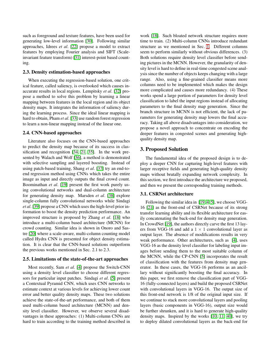
extracting deeper information of saliency as well as main- taining the output resolution. 3.1.1 Dilated convolution One of the critical components of our design is the di- lated convolutional layer. A 2-D dilated convolution can be deﬁned as follow: M N y(m, n) = x(m + r × i, n + r × j)w(i, j) (1) Figure 3. 3 × 3 convolution kernels with different dilation rate as 1, 2, and 3. i=1 j=1 y(m, n) is the output of dilated convolution from input x(m, n) and a ﬁlter w(i, j) with the length and the width of M and N respectively. The parameter r is the dilation rate. If r = 1, a dilated convolution turns into a normal convolution. Dilated convolutional layers have been demonstrated in segmentation tasks with signiﬁcant improvement of accu- racy [10, 11, 40] and it is a good alternative of pooling layer. Although pooling layers (e.g., max and average pool- ing) are widely used for maintaining invariance and con- trolling overﬁtting, they also dramatically reduce the spatial resolution meaning the spatial information of feature map is lost. Deconvolutional layers [41, 42] can alleviate the loss of information, but the additional complexity and ex- ecution latency may not be suitable for all cases. Dilated convolution is a better choice, which uses sparse kernels (as shown in Fig. 3) to alternate the pooling and convolutional layer. This character enlarges the receptive ﬁeld without increasing the number of parameters or the amount of com- putation (e.g., adding more convolutional layers can make larger receptive ﬁelds but introduce more operations). In dilated convolution, a small-size kernel with k × k ﬁlter is enlarged to k + (k − 1)(r − 1) with dilated stride r. Thus it allows ﬂexible aggregation of the multi-scale contextual information while keeping the same resolution. Examples can be found in Fig. 3 where normal convolution gets 3 × 3 receptive ﬁeld and two dilated convolutions deliver 5 × 5 and 7 × 7 receptive ﬁelds respectively. 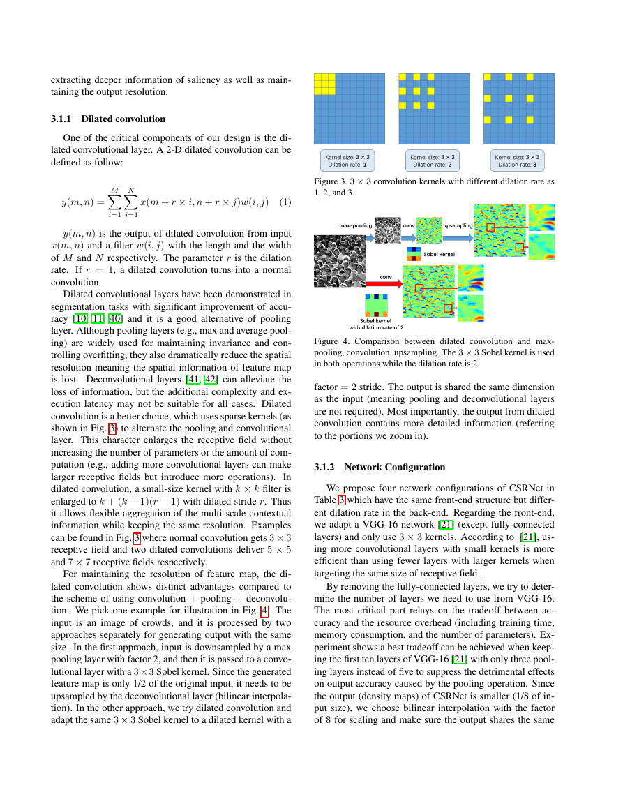For maintaining the resolution of feature map, the di- lated convolution shows distinct advantages compared to the scheme of using convolution + pooling + deconvolu- tion. We pick one example for illustration in Fig. 4. The input is an image of crowds, and it is processed by two approaches separately for generating output with the same size. In the ﬁrst approach, input is downsampled by a max pooling layer with factor 2, and then it is passed to a convo- lutional layer with a 3× 3 Sobel kernel. Since the generated feature map is only 1/2 of the original input, it needs to be upsampled by the deconvolutional layer (bilinear interpola- tion). In the other approach, we try dilated convolution and adapt the same 3 × 3 Sobel kernel to a dilated kernel with a Figure 4. Comparison between dilated convolution and max- pooling, convolution, upsampling. The 3 × 3 Sobel kernel is used in both operations while the dilation rate is 2. factor = 2 stride. The output is shared the same dimension as the input (meaning pooling and deconvolutional layers are not required). Most importantly, the output from dilated convolution contains more detailed information (referring to the portions we zoom in). 3.1.2 Network Conﬁguration We propose four network conﬁgurations of CSRNet in Table 3 which have the same front-end structure but differ- ent dilation rate in the back-end. Regarding the front-end, we adapt a VGG-16 network [21] (except fully-connected layers) and only use 3 × 3 kernels. According to [21], us- ing more convolutional layers with small kernels is more efﬁcient than using fewer layers with larger kernels when targeting the same size of receptive ﬁeld . By removing the fully-connected layers, we try to deter- mine the number of layers we need to use from VGG-16. The most critical part relays on the tradeoff between ac- curacy and the resource overhead (including training time, memory consumption, and the number of parameters). Ex- periment shows a best tradeoff can be achieved when keep- ing the ﬁrst ten layers of VGG-16 [21] with only three pool- ing layers instead of ﬁve to suppress the detrimental effects on output accuracy caused by the pooling operation. Since the output (density maps) of CSRNet is smaller (1/8 of in- put size), we choose bilinear interpolation with the factor of 8 for scaling and make sure the output shares the same

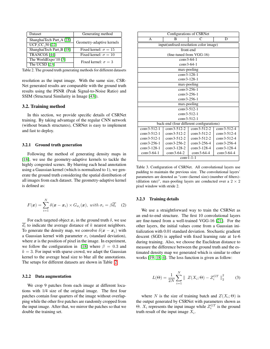
Dataset ShanghaiTech Part A [18] UCF CC 50 [22] ShanghaiTech Part B [18] TRANCOS [44] The WorldExpo’10 [3] The UCSD [23] Generating method Geometry-adaptive kernels Fixed kernel: σ = 15 Fixed kernel: σ = 10 Fixed kernel: σ = 3 Table 2. The ground truth generating methods for different datasets resolution as the input image. With the same size, CSR- Net generated results are comparable with the ground truth results using the PSNR (Peak Signal-to-Noise Ratio) and SSIM (Structural Similarity in Image [43]). 3.2. Training method In this section, we provide speciﬁc details of CSRNet training. By taking advantage of the regular CNN network (without branch structures), CSRNet is easy to implement and fast to deploy. 3.2.1 Ground truth generation Following the method of generating density maps in [18], we use the geometry-adaptive kernels to tackle the highly congested scenes. By blurring each head annotation using a Gaussian kernel (which is normalized to 1), we gen- erate the ground truth considering the spatial distribution of all images from each dataset. The geometry-adaptive kernel is deﬁned as: N i=1 F (x) = δ(x − xi) × Gσi(x), with σi = βdi (2) For each targeted object xi in the ground truth δ, we use di to indicate the average distance of k nearest neighbors. To generate the density map, we convolve δ(x − xi) with a Gaussian kernel with parameter σi (standard deviation), where x is the position of pixel in the image. In experiment, we follow the conﬁguration in [18] where β = 0.3 and k = 3. For input with sparse crowd, we adapt the Gaussian kernel to the average head size to blur all the annotations. The setups for different datasets are shown in Table 2. 3.2.2 Data augmentation We crop 9 patches from each image at different loca- tions with 1/4 size of the original image. The ﬁrst four patches contain four quarters of the image without overlap- ping while the other ﬁve patches are randomly cropped from the input image. After that, we mirror the patches so that we double the training set. Conﬁgurations of CSRNet A B C D input(unﬁxed-resolution color image) front-end (ﬁne-tuned from VGG-16) conv3-64-1 conv3-64-1 max-pooling conv3-128-1 conv3-128-1 max-pooling conv3-256-1 conv3-256-1 conv3-256-1 max-pooling conv3-512-1 conv3-512-1 conv3-512-1 back-end (four different conﬁgurations) conv3-512-1 conv3-512-1 conv3-512-1 conv3-256-1 conv3-128-1 conv3-64-1 conv3-512-2 conv3-512-2 conv3-512-2 conv3-256-2 conv3-128-2 conv3-64-2 conv3-512-2 conv3-512-2 conv3-512-2 conv3-256-4 conv3-128-4 conv3-64-4 conv3-512-4 conv3-512-4 conv3-512-4 conv3-256-4 conv3-128-4 conv3-64-4 conv1-1-1 Table 3. Conﬁguration of CSRNet. All convolutional layers use padding to maintain the previous size. The convolutional layers’ parameters are denoted as “conv-(kernel size)-(number of ﬁlters)- (dilation rate)”, max-pooling layers are conducted over a 2 × 2 pixel window with stride 2. 3.2.3 Training details We use a straightforward way to train the CSRNet as an end-to-end structure. The ﬁrst 10 convolutional layers are ﬁne-tuned from a well-trained VGG-16 [21]. For the other layers, the initial values come from a Gaussian ini- tialization with 0.01 standard deviation. Stochastic gradient descent (SGD) is applied with ﬁxed learning rate at 1e-6 during training. Also, we choose the Euclidean distance to measure the difference between the ground truth and the es- timated density map we generated which is similar to other works [19, 18, 4]. The loss function is given as follow: N i=1 L(Θ) = 1 2N Z(Xi; Θ) − Z GT i 2 2 (3) where N is the size of training batch and Z(Xi; Θ) is the output generated by CSRNet with parameters shown as Θ. Xi represents the input image while Z GT is the ground truth result of the input image Xi. i

4. Experiments We demonstrate our approach in ﬁve different public datasets [18, 3, 22, 23, 44]. Compared to the previous state- of-the-art methods [4, 5], our model is smaller, more accu- rate, and easier to train and deploy. In this section, the eval- uation metrics are introduced, and then an ablation study of ShanghaiTech Part A dataset is conducted to analyze the conﬁguration of our model (shown in Table 3). Along with the ablation study, we evaluate and compare our proposed method to the previous state-of-the-art methods in all these ﬁve datasets. The implementation of our model is based on the Caffe framework [13]. 4.1. Evaluation metrics The MAE and the MSE are used for evaluation which are deﬁned as: N N i=1 i=1 1 N 1 N M AE = M SE = | Ci − C GT i | | Ci − C GT i |2 (4) (5) L W where N is the number of images in one test sequence is the ground truth of counting. Ci represents the and C GT estimated count which is deﬁned as follows: i Ci = zl,w (6) l=1 w=1 L and W show the length and width of the density map respectively while zl,w is the pixel at (l, w) of the generated density map. Ci means the estimated counting number for image Xi. We also use the PSNR and SSIM to evaluate the quality of the output density map on ShanghaiTech Part A dataset. To calculate the PSNR and SSIM, we follow the preprocess given by [5], which includes the density map resizing (same size with the original input) with interpolation and normal- ization for both ground truth and predicted density map. 4.2. Ablations on ShanghaiTech Part A In this subsection, we perform an ablation study to an- alyze the four conﬁgurations of the CSRNet on Shang- haiTech Part A dataset [18] which is a new large-scale crowd counting dataset including 482 images for congested scenes with 241,667 annotated persons. It is challenging to count from these images because of the extremely con- gested scenes, the varied perspective, and the unﬁxed res- olution. These four conﬁgurations are shown in Table 3. CSRNet A is the network with all the dilation rate of 1. 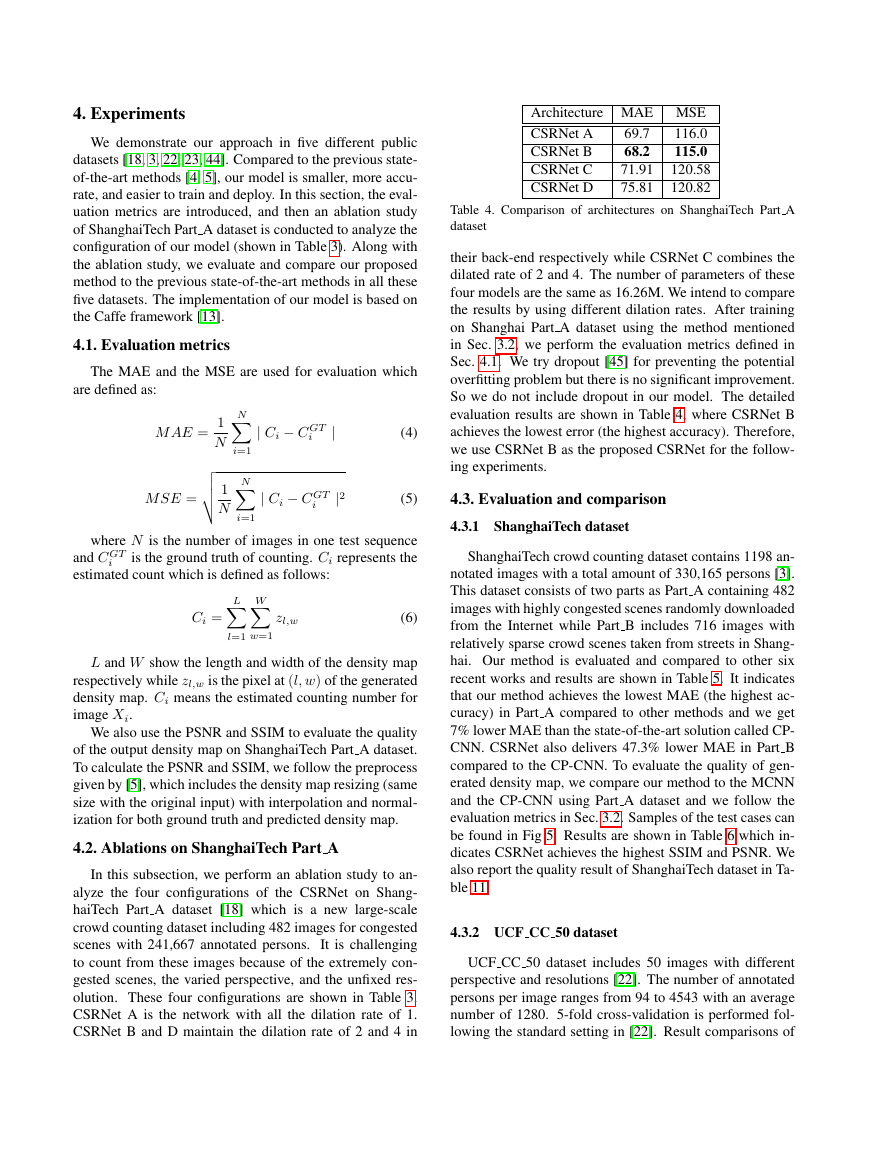CSRNet B and D maintain the dilation rate of 2 and 4 in Architecture MAE MSE 116.0 CSRNet A 115.0 CSRNet B 120.58 CSRNet C CSRNet D 120.82 69.7 68.2 71.91 75.81 Table 4. Comparison of architectures on ShanghaiTech Part A dataset their back-end respectively while CSRNet C combines the dilated rate of 2 and 4. The number of parameters of these four models are the same as 16.26M. We intend to compare the results by using different dilation rates. After training on Shanghai Part A dataset using the method mentioned in Sec. 3.2, we perform the evaluation metrics deﬁned in Sec. 4.1. We try dropout [45] for preventing the potential overﬁtting problem but there is no signiﬁcant improvement. So we do not include dropout in our model. The detailed evaluation results are shown in Table 4, where CSRNet B achieves the lowest error (the highest accuracy). Therefore, we use CSRNet B as the proposed CSRNet for the follow- ing experiments. 4.3. Evaluation and comparison 4.3.1 ShanghaiTech dataset ShanghaiTech crowd counting dataset contains 1198 an- notated images with a total amount of 330,165 persons [3]. This dataset consists of two parts as Part A containing 482 images with highly congested scenes randomly downloaded from the Internet while Part B includes 716 images with relatively sparse crowd scenes taken from streets in Shang- hai. Our method is evaluated and compared to other six recent works and results are shown in Table 5. It indicates that our method achieves the lowest MAE (the highest ac- curacy) in Part A compared to other methods and we get 7% lower MAE than the state-of-the-art solution called CP- CNN. CSRNet also delivers 47.3% lower MAE in Part B compared to the CP-CNN. To evaluate the quality of gen- erated density map, we compare our method to the MCNN and the CP-CNN using Part A dataset and we follow the evaluation metrics in Sec. 3.2. Samples of the test cases can be found in Fig 5. Results are shown in Table 6 which in- dicates CSRNet achieves the highest SSIM and PSNR. We also report the quality result of ShanghaiTech dataset in Ta- ble 11. 4.3.2 UCF CC 50 dataset UCF CC 50 dataset includes 50 images with different perspective and resolutions [22]. The number of annotated persons per image ranges from 94 to 4543 with an average number of 1280. 5-fold cross-validation is performed fol- lowing the standard setting in [22]. Result comparisons of

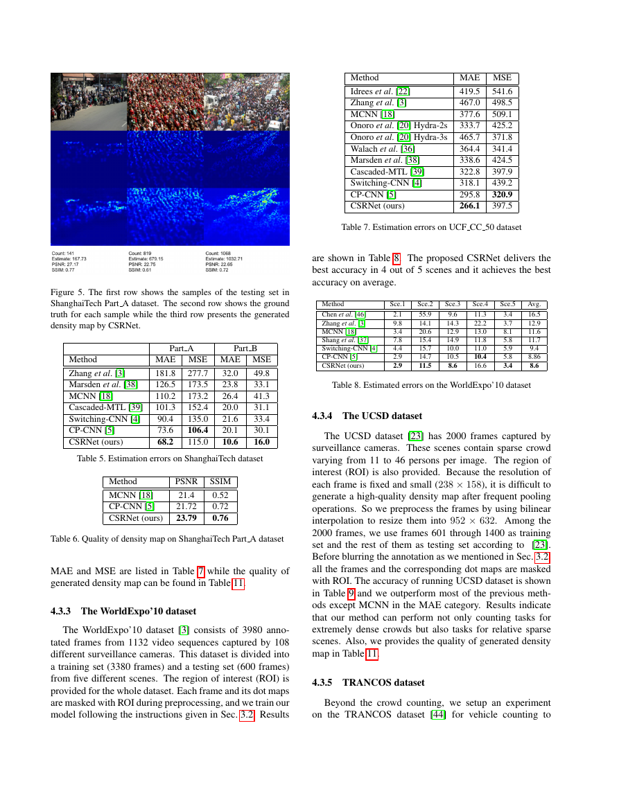
Method Idrees et al. [22] Zhang et al. [3] MCNN [18] Onoro et al. [20] Hydra-2s Onoro et al. [20] Hydra-3s Walach et al. [36] Marsden et al. [38] Cascaded-MTL [39] Switching-CNN [4] CP-CNN [5] CSRNet (ours) MAE MSE 541.6 419.5 498.5 467.0 509.1 377.6 425.2 333.7 465.7 371.8 341.4 364.4 424.5 338.6 397.9 322.8 318.1 439.2 320.9 295.8 266.1 397.5 Table 7. Estimation errors on UCF CC 50 dataset are shown in Table 8. The proposed CSRNet delivers the best accuracy in 4 out of 5 scenes and it achieves the best accuracy on average. Method Chen et al. [46] Zhang et al. [3] MCNN [18] Shang et al. [37] Switching-CNN [4] CP-CNN [5] CSRNet (ours) Sce.1 2.1 9.8 3.4 7.8 4.4 2.9 2.9 Sce.2 55.9 14.1 20.6 15.4 15.7 14.7 11.5 Sce.3 9.6 14.3 12.9 14.9 10.0 10.5 8.6 Sce.4 11.3 22.2 13.0 11.8 11.0 10.4 16.6 Sce.5 3.4 3.7 8.1 5.8 5.9 5.8 3.4 Avg. 16.5 12.9 11.6 11.7 9.4 8.86 8.6 Table 8. Estimated errors on the WorldExpo’10 dataset 4.3.4 The UCSD dataset The UCSD dataset [23] has 2000 frames captured by surveillance cameras. These scenes contain sparse crowd varying from 11 to 46 persons per image. The region of interest (ROI) is also provided. Because the resolution of each frame is ﬁxed and small (238 × 158), it is difﬁcult to generate a high-quality density map after frequent pooling operations. So we preprocess the frames by using bilinear interpolation to resize them into 952 × 632. Among the 2000 frames, we use frames 601 through 1400 as training set and the rest of them as testing set according to [23]. Before blurring the annotation as we mentioned in Sec. 3.2, all the frames and the corresponding dot maps are masked with ROI. The accuracy of running UCSD dataset is shown in Table 9 and we outperform most of the previous meth- ods except MCNN in the MAE category. Results indicate that our method can perform not only counting tasks for extremely dense crowds but also tasks for relative sparse scenes. Also, we provides the quality of generated density map in Table 11. 4.3.5 TRANCOS dataset Beyond the crowd counting, we setup an experiment on the TRANCOS dataset [44] for vehicle counting to Figure 5. The ﬁrst row shows the samples of the testing set in ShanghaiTech Part A dataset. The second row shows the ground truth for each sample while the third row presents the generated density map by CSRNet. Part A Part B Method Zhang et al. [3] Marsden et al. [38] MCNN [18] Cascaded-MTL [39] Switching-CNN [4] CP-CNN [5] CSRNet (ours) MAE MSE MAE MSE 49.8 181.8 126.5 33.1 41.3 110.2 31.1 101.3 33.4 90.4 73.6 30.1 16.0 68.2 277.7 173.5 173.2 152.4 135.0 106.4 115.0 32.0 23.8 26.4 20.0 21.6 20.1 10.6 Table 5. Estimation errors on ShanghaiTech dataset Method MCNN [18] CP-CNN [5] CSRNet (ours) PSNR SSIM 0.52 21.4 0.72 21.72 23.79 0.76 Table 6. Quality of density map on ShanghaiTech Part A dataset MAE and MSE are listed in Table 7 while the quality of generated density map can be found in Table 11. 4.3.3 The WorldExpo’10 dataset The WorldExpo’10 dataset [3] consists of 3980 anno- tated frames from 1132 video sequences captured by 108 different surveillance cameras. This dataset is divided into a training set (3380 frames) and a testing set (600 frames) from ﬁve different scenes. The region of interest (ROI) is provided for the whole dataset. Each frame and its dot maps are masked with ROI during preprocessing, and we train our model following the instructions given in Sec. 3.2. Results

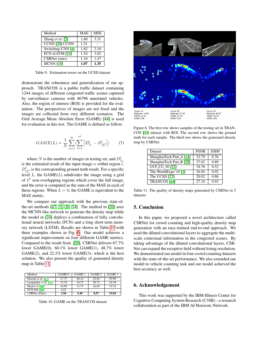
Method Zhang et al. [3] CCNN [20] CCNN Switching-CNN [4] FCN-rLSTM [24] CSRNet (ours) MCNN [18] - MAE MSE 1.60 3.31 1.51 1.62 1.54 1.16 1.07 2.10 3.02 1.47 1.35 Table 9. Estimation errors on the UCSD dataset demonstrate the robustness and generalization of our ap- proach. TRANCOS is a public trafﬁc dataset containing 1244 images of different congested trafﬁc scenes captured by surveillance cameras with 46796 annotated vehicles. Also, the region of interest (ROI) is provided for the eval- uation. The perspectives of images are not ﬁxed and the images are collected from very different scenarios. The Grid Average Mean Absolute Error (GAME) [44] is used for evaluation in this test. The GAME is deﬁned as follow: N ( n=1 4L l=1 1 N GAM E(L) = Dl ) − Dl I gt n In (7) I gt n where N is the number of images in testing set, and Dl In is the estimated result of the input image n within region l. is the corresponding ground truth result. For a speciﬁc Dl level L, the GAME(L) subdivides the image using a grid of 4L non-overlapping regions which cover the full image, and the error is computed as the sum of the MAE in each of these regions. When L = 0, the GAME is equivalent to the MAE metric. We compare our approach with the previous state-of- the-art methods [47, 32, 20, 24]. The method in [20] uses the MCNN-like network to generate the density map while the model in [24] deploys a combination of fully convolu- tional neural networks (FCN) and a long short-term mem- ory network (LSTM). Results are shown in Table 10 with three examples shown in Fig. 6. Our model achieves a signiﬁcant improvement on four different GAME metrics. Compared to the result from [20], CSRNet delivers 67.7% lower GAME(0), 60.1% lower GAME(1), 48.7% lower GAME(2), and 22.2% lower GAME(3), which is the best solution. We also present the quality of generated density map in Table 11. Method Fiaschi et al. [47] Lempitsky et al. [32] Hydra-3s [20] FCN-HA [24] CSRNet (Ours) GAME 0 GAME 1 GAME 2 GAME 3 17.77 13.76 10.99 4.21 3.56 20.14 16.72 13.75 - 5.49 23.65 20.72 16.69 - 8.57 25.99 24.36 19.32 - 15.04 Table 10. GAME on the TRANCOS dataset Figure 6. The ﬁrst row shows samples of the testing set in TRAN- COS [44] dataset with ROI. The second row shows the ground truth for each sample. The third row shows the generated density map by CSRNet. Dataset ShanghaiTech Part A [18] ShanghaiTech Part B [18] UCF CC 50 [22] The WorldExpo’10 [3] The UCSD [23] TRANCOS [44] PSNR SSIM 0.76 23.79 0.89 27.02 18.76 0.52 0.92 26.94 0.86 20.02 27.10 0.93 Table 11. The quality of density maps generated by CSRNet in 5 datasets 5. Conclusion In this paper, we proposed a novel architecture called CSRNet for crowd counting and high-quality density map generation with an easy-trained end-to-end approach. We used the dilated convolutional layers to aggregate the multi- scale contextual information in the congested scenes. By taking advantage of the dilated convolutional layers, CSR- Net can expand the receptive ﬁeld without losing resolution. We demonstrated our model in four crowd counting datasets with the state-of-the-art performance. We also extended our model to vehicle counting task and our model achieved the best accuracy as well. 6. Acknowledgement This work was supported by the IBM-Illinois Center for Cognitive Computing System Research (C3SR) - a research collaboration as part of the IBM AI Horizons Network.

分享到：

赞收藏

资料库

CSRNet网络用于高度拥挤场景.pdf

相关推荐

人工智能

热门标签

最新资料