Mastering the game of Go without human knowledge.pdf

发布时间：2022-05-31 发布人：admin 分类：说明书资料大小：3.84M 资料格式：pdf 举报版权申诉

liuhui516-10031056-4744302543004514268.pdf-第1页.png

第1页 / 共18页

liuhui516-10031056-4744302543004514268.pdf-第2页.png

第2页 / 共18页

liuhui516-10031056-4744302543004514268.pdf-第3页.png

第3页 / 共18页

liuhui516-10031056-4744302543004514268.pdf-第4页.png

第4页 / 共18页

liuhui516-10031056-4744302543004514268.pdf-第5页.png

第5页 / 共18页

liuhui516-10031056-4744302543004514268.pdf-第6页.png

第6页 / 共18页

liuhui516-10031056-4744302543004514268.pdf-第7页.png

第7页 / 共18页

liuhui516-10031056-4744302543004514268.pdf-第8页.png

第8页 / 共18页

Mastering the game of Go without human knowledge

Authors

Abstract

Reinforcement learning in AlphaGo Zero

Empirical analysis of AlphaGo Zero training

Knowledge learned by AlphaGo Zero

Final performance of AlphaGo Zero

Conclusion

References

Acknowledgements

Author Contributions

Figure 1 Self-play reinforcement learning in AlphaGo Zero.

Figure 2 MCTS in AlphaGo Zero.

Figure 3 Empirical evaluation of AlphaGo Zero.

Figure 4 Comparison of neural network architectures in AlphaGo Zero and AlphaGo Lee.

Figure 5 Go knowledge learned by AlphaGo Zero.

Figure 6 Performance of AlphaGo Zero.

Extended Data Figure 1 Tournament games between AlphaGo Zero (20 blocks, 3 days) versus AlphaGo Lee using 2 h time controls.

Extended Data Figure 2 Frequency of occurence over time during training, for each joseki from Fig.

Extended Data Figure 3 Frequency of occurence over time during training, for each joseki from Fig.

Extended Data Figure 4 AlphaGo Zero (20 blocks) self-play games.

Extended Data Figure 5 AlphaGo Zero (40 blocks) self-play games.

Extended Data Figure 6 AlphaGo Zero (40 blocks, 40 days) versus AlphaGo Master tournament games using 2 h time controls.

Extended Data Table 1Move prediction accuracy.

Extended Data Table 2Game outcome prediction error.

Extended Data Table 3Learning rate schedule.

ARTicLE Mastering the game of Go without human knowledge David Silver1*, Julian Schrittwieser1*, Karen Simonyan1*, ioannis Antonoglou1, Aja Huang1, Arthur Guez1, Thomas Hubert1, Lucas baker1, Matthew Lai1, Adrian bolton1, Yutian chen1, Timothy Lillicrap1, Fan Hui1, Laurent Sifre1, George van den Driessche1, Thore Graepel1 & Demis Hassabis1 doi:10.1038/nature24270 A long-standing goal of artificial intelligence is an algorithm that learns, tabula rasa, superhuman proficiency in challenging domains. Recently, AlphaGo became the first program to defeat a world champion in the game of Go. The tree search in AlphaGo evaluated positions and selected moves using deep neural networks. These neural networks were trained by supervised learning from human expert moves, and by reinforcement learning from self-play. Here we introduce an algorithm based solely on reinforcement learning, without human data, guidance or domain knowledge beyond game rules. AlphaGo becomes its own teacher: a neural network is trained to predict AlphaGo’s own move selections and also the winner of AlphaGo’s games. This neural network improves the strength of the tree search, resulting in higher quality move selection and stronger self-play in the next iteration. Starting tabula rasa, our new program AlphaGo Zero achieved superhuman performance, winning 100–0 against the previously published, champion-defeating AlphaGo. Much progress towards artificial intelligence has been made using supervised learning systems that are trained to replicate the decisions of human experts1–4. However, expert data sets are often expensive, unreliable or simply unavailable. Even when reliable data sets are available, they may impose a ceiling on the performance of systems trained in this manner5. By contrast, reinforcement learning systems are trained from their own experience, in principle allowing them to exceed human capabilities, and to operate in domains where human expertise is lacking. Recently, there has been rapid progress towards this goal, using deep neural networks trained by reinforcement learning. These systems have outperformed humans in computer games, such as Atari6,7 and 3D virtual environments8–10. However, the most chal lenging domains in terms of human intellect—such as the game of Go, widely viewed as a grand challenge for artificial intelligence11—require a precise and sophisticated lookahead in vast search spaces. Fully gene ral methods have not previously achieved humanlevel performance in these domains. AlphaGo was the first program to achieve superhuman performance in Go. The published version12, which we refer to as AlphaGo Fan, defeated the European champion Fan Hui in October 2015. AlphaGo Fan used two deep neural networks: a policy network that outputs move probabilities and a value network that outputs a position eval uation. The policy network was trained initially by supervised learn ing to accurately predict human expert moves, and was subsequently refined by policygradient reinforcement learning. The value network was trained to predict the winner of games played by the policy net work against itself. Once trained, these networks were combined with a Monte Carlo tree search (MCTS)13–15 to provide a lookahead search, using the policy network to narrow down the search to highprobability moves, and using the value network (in conjunction with Monte Carlo rollouts using a fast rollout policy) to evaluate positions in the tree. A subsequent version, which we refer to as AlphaGo Lee, used a similar approach (see Methods), and defeated Lee Sedol, the winner of 18 inter national titles, in March 2016. Our program, AlphaGo Zero, differs from AlphaGo Fan and AlphaGo Lee12 in several important aspects. First and foremost, it is trained solely by selfplay reinforcement learning, starting from ran dom play, without any supervision or use of human data. Second, it uses only the black and white stones from the board as input features. Third, it uses a single neural network, rather than separate policy and value networks. Finally, it uses a simpler tree search that relies upon this single neural network to evaluate positions and sample moves, without performing any Monte Carlo rollouts. To achieve these results, we introduce a new reinforcement learning algorithm that incorporates lookahead search inside the training loop, resulting in rapid improve ment and precise and stable learning. Further technical differences in the search algorithm, training procedure and network architecture are described in Methods. Reinforcement learning in AlphaGo Zero Our new method uses a deep neural network fθ with parameters θ. This neural network takes as an input the raw board representation s of the position and its history, and outputs both move probabilities and a value, (p, v) = fθ(s). The vector of move probabilities p represents the probability of selecting each move a (including pass), pa = Pr(a| s). The value v is a scalar evaluation, estimating the probability of the current player winning from position s. This neural network combines the roles of both policy network and value network12 into a single architecture. The neural network consists of many residual blocks4 of convolutional layers16,17 with batch normalization18 and rectifier nonlinearities19 (see Methods). The neural network in AlphaGo Zero is trained from games of self play by a novel reinforcement learning algorithm. In each position s, an MCTS search is executed, guided by the neural network fθ. The MCTS search outputs probabilities π of playing each move. These search probabilities usually select much stronger moves than the raw move probabilities p of the neural network fθ(s); MCTS may therefore be viewed as a powerful policy improvement operator20,21. Selfplay with search—using the improved MCTSbased policy to select each move, then using the game winner z as a sample of the value—may be viewed as a powerful policy evaluation operator. The main idea of our reinforcement learning algorithm is to use these search operators 1DeepMind, 5 New Street Square, London EC4A 3TW, UK. *These authors contributed equally to this work. 3 5 4 | N A T U R E | V O L 5 5 0 | 1 9 O c T O b E R 2 0 1 7 © 2017 Macmillan Publishers Limited, part of Springer Nature. All rights reserved.

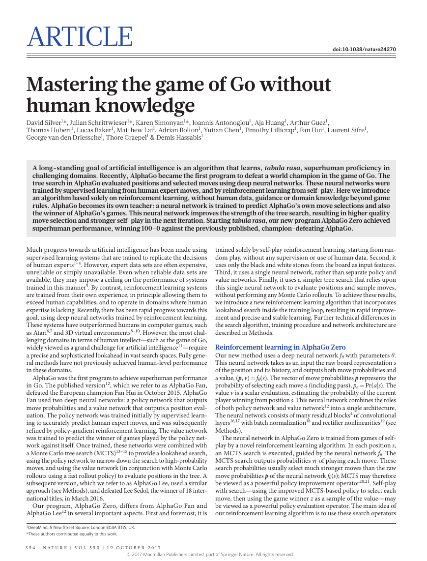
a Self-play s1 a1 ~ 1 1 b Neural network training s1 s2 2 s2 a2 ~ 2 s3 at ~ t 3 s3 f f f p1 1 v1 p2 2 v2 p3 3 v3 sT z z Figure 1 | Self-play reinforcement learning in AlphaGo Zero. a, The program plays a game s1, ..., sT against itself. In each position st, an MCTS αθ is executed (see Fig. 2) using the latest neural network fθ. Moves are selected according to the search probabilities computed by the MCTS, at ∼ πt. The terminal position sT is scored according to the rules of the game to compute the game winner z. b, Neural network training in AlphaGo Zero. The neural network takes the raw board position st as its input, passes it through many convolutional layers with parameters θ, and outputs both a vector pt, representing a probability distribution over moves, and a scalar value vt, representing the probability of the current player winning in position st. The neural network parameters θ are updated to maximize the similarity of the policy vector pt to the search probabilities πt, and to minimize the error between the predicted winner vt and the game winner z (see equation (1)). The new parameters are used in the next iteration of selfplay as in a. repeatedly in a policy iteration procedure22,23: the neural network’s parameters are updated to make the move probabilities and value (p, v) = fθ(s) more closely match the improved search probabilities and self play winner (π, z); these new parameters are used in the next iteration of selfplay to make the search even stronger. Figure 1 illustrates the selfplay training pipeline. 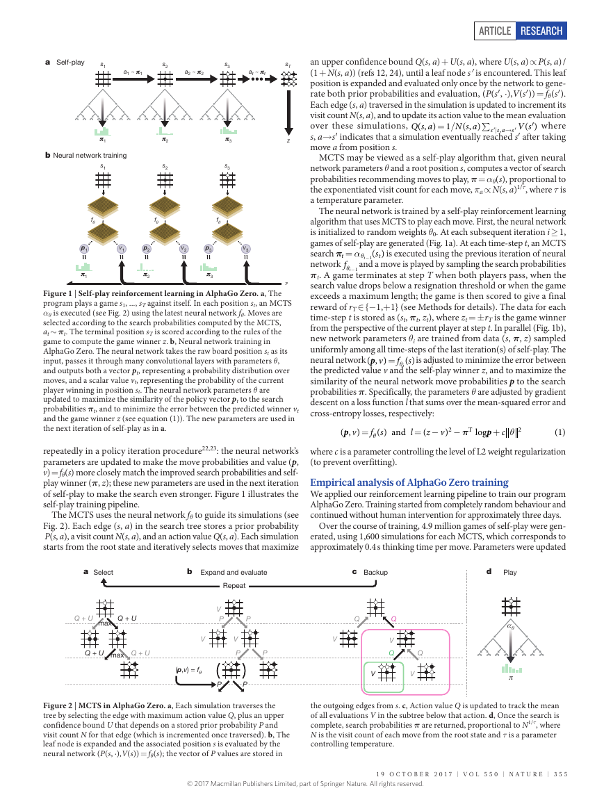The MCTS uses the neural network fθ to guide its simulations (see Fig. 2). Each edge (s, a) in the search tree stores a prior probability P(s, a), a visit count N(s, a), and an action value Q(s, a). Each simulation starts from the root state and iteratively selects moves that maximize an upper confidence bound Q(s, a) + U(s, a), where U(s, a) ∝ P(s, a) / (1 + N(s, a)) (refs 12, 24), until a leaf node s′ is encountered. This leaf position is expanded and evaluated only once by the network to gene rate both prior probabilities and evaluation, (P(s′ , ·),V(s′ )) = fθ(s′ ). Each edge (s, a) traversed in the simulation is updated to increment its visit count N(s, a), and to update its action value to the mean evaluation over these simulations, where s, a→ s′ indicates that a simulation eventually reached s′ after taking move a from position s. MCTS may be viewed as a selfplay algorithm that, given neural network parameters θ and a root position s, computes a vector of search probabilities recommending moves to play, π = αθ(s), proportional to the exponentiated visit count for each move, πa ∝ N(s, a)1/τ, where τ is a temperature parameter. N s a ( , ) Q s a ( , ) V s ( ) ′ 1 = / s s a , | →′ ∑ s ′ The neural network is trained by a selfplay reinforcement learning algorithm that uses MCTS to play each move. First, the neural network is initialized to random weights θ0. At each subsequent iteration i ≥ 1, games of selfplay are generated (Fig. 1a). At each timestep t, an MCTS search π α= θ − s( ) is executed using the previous iteration of neural t network θ −f i 1 and a move is played by sampling the search probabilities πt. A game terminates at step T when both players pass, when the search value drops below a resignation threshold or when the game exceeds a maximum length; the game is then scored to give a final reward of rT ∈ {− 1,+ 1} (see Methods for details). The data for each timestep t is stored as (st, πt, zt), where zt = ± rT is the game winner from the perspective of the current player at step t. In parallel (Fig. 1b), new network parameters θi are trained from data (s, π, z) sampled uniformly among all timesteps of the last iteration(s) of selfplay. The neural network is adjusted to minimize the error between the predicted value v and the selfplay winner z, and to maximize the similarity of the neural network move probabilities p to the search probabilities π. Specifically, the parameters θ are adjusted by gradient descent on a loss function l that sums over the meansquared error and crossentropy losses, respectively: z ( (1) where c is a parameter controlling the level of L2 weight regularization (to prevent overfitting). s ( ) and = − p v ( , ) p v ( , ) f = θ log s ( ) T π = − 2 v ) f θ i 1 p + c 2 θ t i l Empirical analysis of AlphaGo Zero training We applied our reinforcement learning pipeline to train our program AlphaGo Zero. Training started from completely random behaviour and continued without human intervention for approximately three days. Over the course of training, 4.9 million games of selfplay were gen erated, using 1,600 simulations for each MCTS, which corresponds to approximately 0.4 s thinking time per move. Parameters were updated a Select b Expand and evaluate c Backup d Play Q + U max Q + U Q + U max Q + U Repeat V P P V V P P (p,v) = f P P Q V Q V Q Q V V Figure 2 | MCTS in AlphaGo Zero. a, Each simulation traverses the tree by selecting the edge with maximum action value Q, plus an upper confidence bound U that depends on a stored prior probability P and visit count N for that edge (which is incremented once traversed). b, The leaf node is expanded and the associated position s is evaluated by the neural network (P(s, ·),V(s)) = fθ(s); the vector of P values are stored in the outgoing edges from s. c, Action value Q is updated to track the mean of all evaluations V in the subtree below that action. d, Once the search is complete, search probabilities π are returned, proportional to N1/τ, where N is the visit count of each move from the root state and τ is a parameter controlling temperature. 1 9 O c T O b E R 2 0 1 7 | V O L 5 5 0 | N A T U R E | 3 5 5 ArticlereSeArcH© 2017 Macmillan Publishers Limited, part of Springer Nature. All rights reserved.

a g n i t a r o E l 5,000 4,000 3,000 2,000 1,000 0 –1,000 –2,000 –3,000 –4,000 b ) % ( s e v o m i l a n o s s e f o r p n o y c a r u c c a n o i t c d e r P i Reinforcement learning Supervised learning AlphaGo Lee 70 60 50 40 30 20 10 0 c l i a n o s s e f o r p f o E S M s e m o c t u o e m a g 0.35 0.30 0.25 0.20 0.15 Reinforcement learning Supervised learning Reinforcement learning Supervised learning 0 10 20 30 40 50 60 70 0 10 20 30 40 50 60 70 0 10 20 30 40 50 60 70 Training time (h) Training time (h) Training time (h) 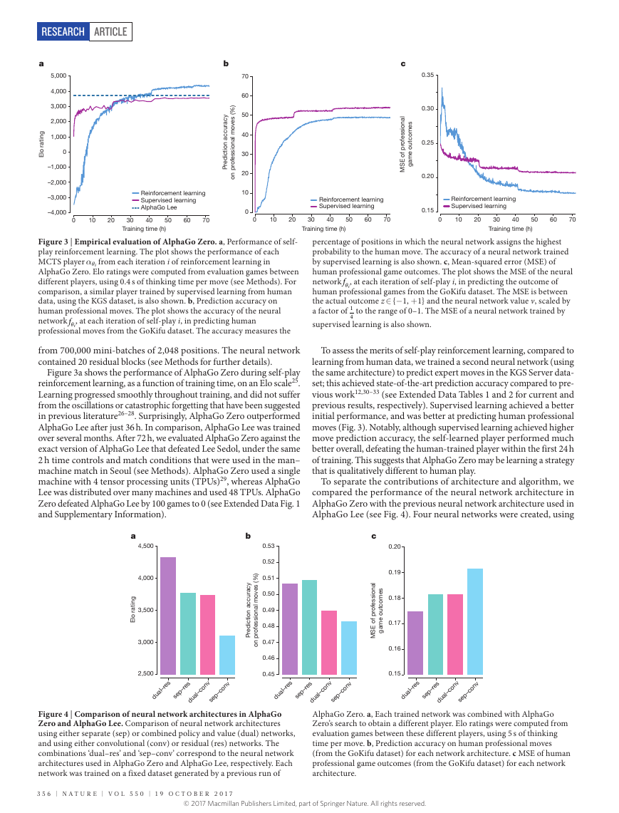Figure 3 | Empirical evaluation of AlphaGo Zero. a, Performance of self play reinforcement learning. The plot shows the performance of each MCTS player αθi from each iteration i of reinforcement learning in AlphaGo Zero. Elo ratings were computed from evaluation games between different players, using 0.4 s of thinking time per move (see Methods). For comparison, a similar player trained by supervised learning from human data, using the KGS dataset, is also shown. b, Prediction accuracy on human professional moves. The plot shows the accuracy of the neural network θf i, at each iteration of selfplay i, in predicting human professional moves from the GoKifu dataset. The accuracy measures the percentage of positions in which the neural network assigns the highest probability to the human move. The accuracy of a neural network trained by supervised learning is also shown. c, Meansquared error (MSE) of human professional game outcomes. The plot shows the MSE of the neural network θf i, at each iteration of selfplay i, in predicting the outcome of human professional games from the GoKifu dataset. The MSE is between the actual outcome z ∈ {− 1, + 1} and the neural network value v, scaled by a factor of 1 to the range of 0–1. The MSE of a neural network trained by 4 supervised learning is also shown. from 700,000 minibatches of 2,048 positions. The neural network contained 20 residual blocks (see Methods for further details). Figure 3a shows the performance of AlphaGo Zero during selfplay reinforcement learning, as a function of training time, on an Elo scale25. Learning progressed smoothly throughout training, and did not suffer from the oscillations or catastrophic forgetting that have been suggested in previous literature26–28. Surprisingly, AlphaGo Zero outperformed AlphaGo Lee after just 36 h. In comparison, AlphaGo Lee was trained over several months. After 72 h, we evaluated AlphaGo Zero against the exact version of AlphaGo Lee that defeated Lee Sedol, under the same 2 h time controls and match conditions that were used in the man– machine match in Seoul (see Methods). AlphaGo Zero used a single machine with 4 tensor processing units (TPUs)29, whereas AlphaGo Lee was distributed over many machines and used 48 TPUs. AlphaGo Zero defeated AlphaGo Lee by 100 games to 0 (see Extended Data Fig. 1 and Supplementary Information). To assess the merits of selfplay reinforcement learning, compared to learning from human data, we trained a second neural network (using the same architecture) to predict expert moves in the KGS Server data set; this achieved stateoftheart prediction accuracy compared to pre vious work12,30–33 (see Extended Data Tables 1 and 2 for current and previous results, respectively). Supervised learning achieved a better initial performance, and was better at predicting human professional moves (Fig. 3). Notably, although supervised learning achieved higher move prediction accuracy, the selflearned player performed much better overall, defeating the humantrained player within the first 24 h of training. This suggests that AlphaGo Zero may be learning a strategy that is qualitatively different to human play. To separate the contributions of architecture and algorithm, we compared the performance of the neural network architecture in AlphaGo Zero with the previous neural network architecture used in AlphaGo Lee (see Fig. 4). 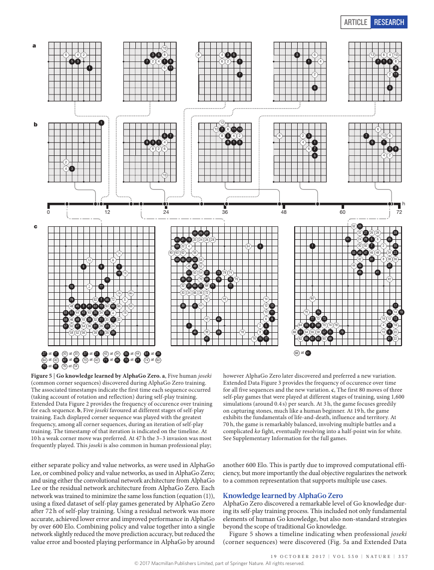Four neural networks were created, using b y c a r u c c a n o i t c d e r P i a 4,500 4,000 g n i t a r o E l 3,500 3,000 2,500 ) % ( s e v o m i l a n o s s e f o r p n o 0.53 0.52 0.51 0.50 0.49 0.48 0.47 0.46 0.45 c l i a n o s s e f o r p f o E S M s e m o c t u o e m a g 0.20 0.19 0.18 0.17 0.16 0.15 sep–res dual–res sep–conv dual–conv dual–res Figure 4 | Comparison of neural network architectures in AlphaGo Zero and AlphaGo Lee. Comparison of neural network architectures using either separate (sep) or combined policy and value (dual) networks, and using either convolutional (conv) or residual (res) networks. The combinations ‘dual–res’ and ‘sep–conv’ correspond to the neural network architectures used in AlphaGo Zero and AlphaGo Lee, respectively. Each network was trained on a fixed dataset generated by a previous run of sep–res dual–conv sep–conv dual–res sep–res dual–conv sep–conv AlphaGo Zero. a, Each trained network was combined with AlphaGo Zero’s search to obtain a different player. Elo ratings were computed from evaluation games between these different players, using 5 s of thinking time per move. b, Prediction accuracy on human professional moves (from the GoKifu dataset) for each network architecture. c MSE of human professional game outcomes (from the GoKifu dataset) for each network architecture. 3 5 6 | N A T U R E | V O L 5 5 0 | 1 9 O c T O b E R 2 0 1 7 ArticlereSeArcH© 2017 Macmillan Publishers Limited, part of Springer Nature. All rights reserved.

a b 2 4 3 0 c 12 6 1 4 5 7 10 8 9 2 11 3 6 7 10 8 5 1 4 9 3 2 60 51 h 72 52 53 44 33 32 24 30 49 42 43 45 27 29 50 47 26 28 5 7 46 31 6 48 41 39 35 23 36 2 8 25 34 38 37 40 4 6 2 5 1 7 5 1 80 76 55 54 65 75 77 72 73 3 56 67 59 58 63 70 57 60 74 71 69 66 64 61 62 78 79 68 at 61 17 14 15 19 16 12 13 4 11 10 9 18 20 21 22 6 2 4 3 5 1 3 2 5 4 7 10 8 1 6 9 11 8 5 4 6 3 2 1 7 3 1 1 12 7 5 4 6 9 3 8 1 2 10 24 10 12 7 8 6 5 9 11 13 4 1 2 3 8 2 4 3 6 36 48 12 5 15 79 48 51 46 50 58 53 59 57 45 44 49 47 52 3 43 10 54 56 2 41 40 39 36 62 63 35 32 31 38 8 14 1 19 18 11 65 60 25 20 80 68 78 66 6 16 72 69 4 17 22 23 24 26 29 9 77 7 13 34 21 28 33 61 59 60 63 80 21 22 62 55 35 32 30 39 23 19 20 25 24 27 26 28 4 57 56 53 48 49 51 33 31 34 50 65 66 58 52 54 70 37 69 73 79 67 68 71 36 72 42 78 74 75 76 77 46 41 44 1 45 43 29 40 38 47 64 3 14 12 13 10 11 9 6 5 7 2 8 16 15 17 18 27 at 17 64 at 40 75 at 39 30 at 20 67 at 39 76 at 34 37 at 21 70 at 40 42 at 34 71 at 25 55 at 44 73 at 21 61 at 39 74 at 60 Figure 5 | Go knowledge learned by AlphaGo Zero. a, Five human joseki (common corner sequences) discovered during AlphaGo Zero training. The associated timestamps indicate the first time each sequence occurred (taking account of rotation and reflection) during selfplay training. Extended Data Figure 2 provides the frequency of occurence over training for each sequence. b, Five joseki favoured at different stages of selfplay training. Each displayed corner sequence was played with the greatest frequency, among all corner sequences, during an iteration of selfplay training. The timestamp of that iteration is indicated on the timeline. At 10 h a weak corner move was preferred. At 47 h the 3–3 invasion was most frequently played. This joseki is also common in human professional play; however AlphaGo Zero later discovered and preferred a new variation. Extended Data Figure 3 provides the frequency of occurence over time for all five sequences and the new variation. c, The first 80 moves of three selfplay games that were played at different stages of training, using 1,600 simulations (around 0.4 s) per search. At 3 h, the game focuses greedily on capturing stones, much like a human beginner. At 19 h, the game exhibits the fundamentals of lifeanddeath, influence and territory. At 70 h, the game is remarkably balanced, involving multiple battles and a complicated ko fight, eventually resolving into a halfpoint win for white. See Supplementary Information for the full games. either separate policy and value networks, as were used in AlphaGo Lee, or combined policy and value networks, as used in AlphaGo Zero; and using either the convolutional network architecture from AlphaGo Lee or the residual network architecture from AlphaGo Zero. Each network was trained to minimize the same loss function (equation (1)), using a fixed dataset of selfplay games generated by AlphaGo Zero after 72 h of selfplay training. Using a residual network was more accurate, achieved lower error and improved performance in AlphaGo by over 600 Elo. Combining policy and value together into a single network slightly reduced the move prediction accuracy, but reduced the value error and boosted playing performance in AlphaGo by around another 600 Elo. This is partly due to improved computational effi ciency, but more importantly the dual objective regularizes the network to a common representation that supports multiple use cases. Knowledge learned by AlphaGo Zero AlphaGo Zero discovered a remarkable level of Go knowledge dur ing its selfplay training process. This included not only fundamental elements of human Go knowledge, but also nonstandard strategies beyond the scope of traditional Go knowledge. Figure 5 shows a timeline indicating when professional joseki (corner sequences) were discovered (Fig. 5a and Extended Data 1 9 O c T O b E R 2 0 1 7 | V O L 5 5 0 | N A T U R E | 3 5 7 ArticlereSeArcH© 2017 Macmillan Publishers Limited, part of Springer Nature. All rights reserved.

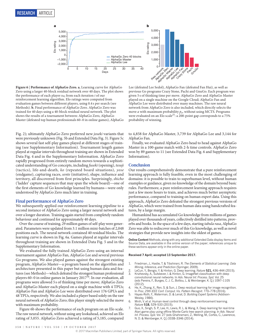
a g n i t a r o E l 5,000 4,000 3,000 2,000 1,000 0 –1,000 –2,000 AlphaGo Zero 40 blocks AlphaGo Master AlphaGo Lee 25 30 35 40 0 5 10 15 20 Days b g n i t a r o E l 5,000 4,000 3,000 2,000 1,000 0 AlphaGo Zero Crazy Stone AlphaGo Fan Pachi GnuGo AlphaGo Lee Raw network AlphaGo M aster Figure 6 | Performance of AlphaGo Zero. a, Learning curve for AlphaGo Zero using a larger 40block residual network over 40 days. The plot shows the performance of each player αθi from each iteration i of our reinforcement learning algorithm. Elo ratings were computed from evaluation games between different players, using 0.4 s per search (see Methods). b, Final performance of AlphaGo Zero. AlphaGo Zero was trained for 40 days using a 40block residual neural network. The plot shows the results of a tournament between: AlphaGo Zero, AlphaGo Master (defeated top human professionals 60–0 in online games), AlphaGo Lee (defeated Lee Sedol), AlphaGo Fan (defeated Fan Hui), as well as previous Go programs Crazy Stone, Pachi and GnuGo. Each program was given 5 s of thinking time per move. AlphaGo Zero and AlphaGo Master played on a single machine on the Google Cloud; AlphaGo Fan and AlphaGo Lee were distributed over many machines. The raw neural network from AlphaGo Zero is also included, which directly selects the move a with maximum probability pa, without using MCTS. Programs were evaluated on an Elo scale25: a 200point gap corresponds to a 75% probability of winning. Fig. 2); ultimately AlphaGo Zero preferred new joseki variants that were previously unknown (Fig. 5b and Extended Data Fig. 3). Figure 5c shows several fast selfplay games played at different stages of train ing (see Supplementary Information). Tournament length games played at regular intervals throughout training are shown in Extended Data Fig. 4 and in the Supplementary Information. AlphaGo Zero rapidly progressed from entirely random moves towards a sophisti cated understanding of Go concepts, including fuseki (opening), tesuji (tactics), lifeanddeath, ko (repeated board situations), yose (endgame), capturing races, sente (initiative), shape, influence and territory, all discovered from first principles. Surprisingly, shicho (‘ladder’ capture sequences that may span the whole board)—one of the first elements of Go knowledge learned by humans—were only understood by AlphaGo Zero much later in training. Final performance of AlphaGo Zero We subsequently applied our reinforcement learning pipeline to a second instance of AlphaGo Zero using a larger neural network and over a longer duration. Training again started from completely random behaviour and continued for approximately 40 days. Over the course of training, 29 million games of selfplay were gener ated. Parameters were updated from 3.1 million minibatches of 2,048 positions each. The neural network contained 40 residual blocks. The learning curve is shown in Fig. 6a. Games played at regular intervals throughout training are shown in Extended Data Fig. 5 and in the Supplementary Information. We evaluated the fully trained AlphaGo Zero using an internal tournament against AlphaGo Fan, AlphaGo Lee and several previous Go programs. We also played games against the strongest existing program, AlphaGo Master—a program based on the algorithm and architecture presented in this paper but using human data and fea tures (see Methods)—which defeated the strongest human professional players 60–0 in online games in January 201734. In our evaluation, all programs were allowed 5 s of thinking time per move; AlphaGo Zero and AlphaGo Master each played on a single machine with 4 TPUs; AlphaGo Fan and AlphaGo Lee were distributed over 176 GPUs and 48 TPUs, respectively. We also included a player based solely on the raw neural network of AlphaGo Zero; this player simply selected the move with maximum probability. Figure 6b shows the performance of each program on an Elo scale. The raw neural network, without using any lookahead, achieved an Elo rating of 3,055. AlphaGo Zero achieved a rating of 5,185, compared 3 5 8 | N A T U R E | V O L 5 5 0 | 1 9 O c T O b E R 2 0 1 7 to 4,858 for AlphaGo Master, 3,739 for AlphaGo Lee and 3,144 for AlphaGo Fan. Finally, we evaluated AlphaGo Zero head to head against AlphaGo Master in a 100game match with 2h time controls. AlphaGo Zero won by 89 games to 11 (see Extended Data Fig. 6 and Supplementary Information). Conclusion Our results comprehensively demonstrate that a pure reinforcement learning approach is fully feasible, even in the most challenging of domains: it is possible to train to superhuman level, without human examples or guidance, given no knowledge of the domain beyond basic rules. Furthermore, a pure reinforcement learning approach requires just a few more hours to train, and achieves much better asymptotic performance, compared to training on human expert data. Using this approach, AlphaGo Zero defeated the strongest previous versions of AlphaGo, which were trained from human data using handcrafted fea tures, by a large margin. Humankind has accumulated Go knowledge from millions of games played over thousands of years, collectively distilled into patterns, prov erbs and books. In the space of a few days, starting tabula rasa, AlphaGo Zero was able to rediscover much of this Go knowledge, as well as novel strategies that provide new insights into the oldest of games. Online Content Methods, along with any additional Extended Data display items and Source Data, are available in the online version of the paper; references unique to these sections appear only in the online paper. received 7 April; accepted 13 September 2017. 1. Friedman, J., Hastie, T. & Tibshirani, R. The Elements of Statistical Learning: Data Mining, Inference, and Prediction (Springer, 2009). 2. LeCun, Y., Bengio, Y. & Hinton, G. Deep learning. Nature 521, 436–444 (2015). 3. Krizhevsky, A., Sutskever, I. & Hinton, G. ImageNet classification with deep convolutional neural networks. In Adv. Neural Inf. Process. Syst. Vol. 25 (eds Pereira, F., Burges, C. J. C., Bottou, L. & Weinberger, K. Q.) 1097–1105 (2012). 4. He, K., Zhang, X., Ren, S. & Sun, J. Deep residual learning for image recognition. In Proc. 29th IEEE Conf. Comput. Vis. Pattern Recognit. 770–778 (2016). 5. Hayes-Roth, F., Waterman, D. & Lenat, D. Building Expert Systems (Addison- 6. Mnih, V. et al. Human-level control through deep reinforcement learning. Wesley, 1984). Nature 518, 529–533 (2015). 7. Guo, X., Singh, S. P., Lee, H., Lewis, R. L. & Wang, X. Deep learning for real-time Atari game play using offline Monte-Carlo tree search planning. In Adv. Neural Inf. Process. Syst. Vol. 27 (eds Ghahramani, Z., Welling, M., Cortes, C., Lawrence, N. D. & Weinberger, K. Q.) 3338–3346 (2014). ArticlereSeArcH© 2017 Macmillan Publishers Limited, part of Springer Nature. All rights reserved.

Proc. 33rd Int. Conf. Mach. Learn. Vol. 48 (eds Balcan, M. F. & Weinberger, K. Q.) 1928–1937 (2016). Jaderberg, M. et al. Reinforcement learning with unsupervised auxiliary tasks. In 5th Int. Conf. Learn. Representations (2017). 9. 10. Dosovitskiy, A. & Koltun, V. Learning to act by predicting the future. In 5th Int. Conf. Learn. Representations (2017). 11. Man´dziuk, J. in Challenges for Computational Intelligence (Duch, W. & Man´dziuk, J.) 407–442 (Springer, 2007). 12. Silver, D. et al. Mastering the game of Go with deep neural networks and tree search. Nature 529, 484–489 (2016). 13. Coulom, R. Efficient selectivity and backup operators in Monte-Carlo tree search. In 5th Int. Conf. Computers and Games (eds Ciancarini, P. & van den Herik, H. J.) 72–83 (2006). 14. Kocsis, L. & Szepesvári, C. Bandit based Monte-Carlo planning. In 15th Eu. Conf. Mach. Learn. 282–293 (2006). 15. Browne, C. et al. A survey of Monte Carlo tree search methods. IEEE Trans. Comput. Intell. AI Games 4, 1–49 (2012). 16. Fukushima, K. Neocognitron: a self organizing neural network model for a mechanism of pattern recognition unaffected by shift in position. Biol. Cybern. 36, 193–202 (1980). 17. LeCun, Y. & Bengio, Y. in The Handbook of Brain Theory and Neural Networks Ch. 3 (ed. Arbib, M.) 276–278 (MIT Press, 1995). 18. Ioffe, S. & Szegedy, C. Batch normalization: accelerating deep network training by reducing internal covariate shift. In Proc. 32nd Int. Conf. Mach. Learn. Vol. 37 448–456 (2015). 19. Hahnloser, R. H. R., Sarpeshkar, R., Mahowald, M. A., Douglas, R. J. & Seung, H. S. Digital selection and analogue amplification coexist in a cortex-inspired silicon circuit. Nature 405, 947–951 (2000). 20. Howard, R. Dynamic Programming and Markov Processes (MIT Press, 1960). 21. Sutton, R. & Barto, A. Reinforcement Learning: an Introduction (MIT Press, 1998). 22. Bertsekas, D. P. Approximate policy iteration: a survey and some new methods. J. Control Theory Appl. 9, 310–335 (2011). 23. Scherrer, B. Approximate policy iteration schemes: a comparison. In Proc. 31st Int. Conf. Mach. Learn. Vol. 32 1314–1322 (2014). 24. Rosin, C. D. Multi-armed bandits with episode context. Ann. Math. Artif. Intell. 61, 203–230 (2011). 25. Coulom, R. Whole-history rating: a Bayesian rating system for players of time-varying strength. In Int. Conf. Comput. Games (eds van den Herik, H. J., Xu, X. Ma, Z. & Winands, M. H. M.) Vol. 5131 113–124 (Springer, 2008). 26. Laurent, G. J., Matignon, L. & Le Fort-Piat, N. The world of independent learners is not Markovian. Int. J. Knowledge-Based Intelligent Engineering Systems 15, 55–64 (2011). 8. Mnih, V. et al. Asynchronous methods for deep reinforcement learning. In 27. Foerster, J. N. et al. Stabilising experience replay for deep multi-agent reinforcement learning. In Proc. 34th Int. Conf. Mach. Learn. Vol. 70 1146–1155 (2017). 28. Heinrich, J. & Silver, D. Deep reinforcement learning from self-play in imperfect-information games. In NIPS Deep Reinforcement Learning Workshop (2016). 29. Jouppi, N. P. et al. In-datacenter performance analysis of a Tensor Processing Unit. Proc. 44th Annu. Int. Symp. Comp. Architecture Vol. 17 1–12 (2017). 30. Maddison, C. J., Huang, A., Sutskever, I. & Silver, D. Move evaluation in Go using deep convolutional neural networks. In 3rd Int. Conf. Learn. Representations. (2015). 31. Clark, C. & Storkey, A. J. Training deep convolutional neural networks to play Go. In Proc. 32nd Int. Conf. Mach. Learn. Vol. 37 1766–1774 (2015). 32. Tian, Y. & Zhu, Y. Better computer Go player with neural network and long-term prediction. In 4th Int. Conf. Learn. Representations (2016). 33. Cazenave, T. Residual networks for computer Go. IEEE Trans. Comput. Intell. AI Games https://doi.org/10.1109/TCIAIG.2017.2681042 (2017). 34. Huang, A. AlphaGo master online series of games. https://deepmind.com/ research/AlphaGo/match-archive/master (2017). Supplementary Information is available in the online version of the paper. Acknowledgements We thank A. Cain for work on the visuals; A. Barreto, G. Ostrovski, T. Ewalds, T. Schaul, J. Oh and N. Heess for reviewing the paper; and the rest of the DeepMind team for their support. Author Contributions D.S., J.S., K.S., I.A., A.G., L.S. and T.H. designed and implemented the reinforcement learning algorithm in AlphaGo Zero. A.H., J.S., M.L. and D.S. designed and implemented the search in AlphaGo Zero. L.B., J.S., A.H., F.H., T.H., Y.C. and D.S. designed and implemented the evaluation framework for AlphaGo Zero. D.S., A.B., F.H., A.G., T.L., T.G., L.S., G.v.d.D. and D.H. managed and advised on the project. D.S., T.G. and A.G. wrote the paper. Author Information Reprints and permissions information is available at www.nature.com/reprints. The authors declare no competing financial interests. Readers are welcome to comment on the online version of the paper. Publisher’s note: Springer Nature remains neutral with regard to jurisdictional claims in published maps and institutional affiliations. Correspondence and requests for materials should be addressed to D.S. (davidsilver@google.com). reviewer Information Nature thanks S. Singh and the other anonymous reviewer(s) for their contribution to the peer review of this work. 1 9 O c T O b E R 2 0 1 7 | V O L 5 5 0 | N A T U R E | 3 5 9 ArticlereSeArcH© 2017 Macmillan Publishers Limited, part of Springer Nature. All rights reserved.

MethOdS Reinforcement learning. Policy iteration20,21 is a classic algorithm that generates a sequence of improving policies, by alternating between policy evaluation— estimating the value function of the current policy—and policy improvement— using the current value function to generate a better policy. A simple approach to policy evaluation is to estimate the value function from the outcomes of sampled trajectories35,36. A simple approach to policy improvement is to select actions greedily with respect to the value function20. In large state spaces, approximations are necessary to evaluate each policy and to represent its improvement22,23. Classificationbased reinforcement learning37 improves the policy using a simple Monte Carlo search. Many rollouts are executed for each action; the action with the maximum mean value provides a positive training example, while all other actions provide negative training examples; a policy is then trained to classify actions as positive or negative, and used in subsequent rollouts. This may be viewed as a precursor to the policy component of AlphaGo Zero’s training algorithm when τ→ 0. A more recent instantiation, classificationbased modified policy iteration (CBMPI), also performs policy evaluation by regressing a value function towards truncated rollout values, similar to the value component of AlphaGo Zero; this achieved stateoftheart results in the game of Tetris38. However, this previous work was limited to simple rollouts and linear function approximation using hand crafted features. The AlphaGo Zero selfplay algorithm can similarly be understood as an approximate policy iteration scheme in which MCTS is used for both policy improvement and policy evaluation. Policy improvement starts with a neural network policy, executes an MCTS based on that policy’s recommendations, and then projects the (much stronger) search policy back into the function space of the neural network. Policy evaluation is applied to the (much stronger) search policy: the outcomes of selfplay games are also projected back into the function space of the neural network. These projection steps are achieved by training the neural network parameters to match the search probabilities and selfplay game outcome respectively. Guo et al.7 also project the output of MCTS into a neural network, either by regressing a value network towards the search value, or by classifying the action selected by MCTS. This approach was used to train a neural network for playing Atari games; however, the MCTS was fixed—there was no policy iteration—and did not make any use of the trained networks. Self-play reinforcement learning in games. Our approach is most directly appli cable to Zerosum games of perfect information. We follow the formalism of alter nating Markov games described in previous work12, noting that algorithms based on value or policy iteration extend naturally to this setting39. Selfplay reinforcement learning has previously been applied to the game of Go. NeuroGo40,41 used a neural network to represent a value function, using a sophisticated architecture based on Go knowledge regarding connectivity, terri tory and eyes. This neural network was trained by temporaldifference learning42 to predict territory in games of selfplay, building on previous work43. A related approach, RLGO44, represented the value function instead by a linear combination of features, exhaustively enumerating all 3 × 3 patterns of stones; it was trained by temporaldifference learning to predict the winner in games of selfplay. Both NeuroGo and RLGO achieved a weak amateur level of play. MCTS may also be viewed as a form of selfplay reinforcement learning45. The nodes of the search tree contain the value function for the positions encountered during search; these values are updated to predict the winner of simulated games of selfplay. MCTS programs have previously achieved strong amateur level in Go46,47, but used substantial domain expertise: a fast rollout policy, based on handcrafted features13,48, that evaluates positions by running simulations until the end of the game; and a tree policy, also based on handcrafted features, that selects moves within the search tree47. Selfplay reinforcement learning approaches have achieved high levels of perfor mance in other games: chess49–51, checkers52, backgammon53, othello54, Scrabble55 and most recently poker56. In all of these examples, a value function was trained by regression54–56 or temporaldifference learning49–53 from training data generated by selfplay. The trained value function was used as an evaluation function in an alpha–beta search49–54, a simple Monte Carlo search55,57 or counterfactual regret minimization56. However, these methods used handcrafted input features49–53,56 or handcrafted feature templates54,55. In addition, the learning process used super vised learning to initialize weights58, handselected weights for piece values49,51,52, handcrafted restrictions on the action space56 or used preexisting computer pro grams as training opponents49,50, or to generate game records51. Many of the most successful and widely used reinforcement learning methods were first introduced in the context of Zerosum games: temporaldifference learn ing was first introduced for a checkersplaying program59, while MCTS was intro duced for the game of Go13. However, very similar algorithms have subsequently proven highly effective in video games6–8,10, robotics60, industrial control61–63 and online recommendation systems64,65. AlphaGo versions. We compare three distinct versions of AlphaGo: (1) AlphaGo Fan is the previously published program12 that played against Fan Hui in October 2015. This program was distributed over many machines using 176 GPUs. (2) AlphaGo Lee is the program that defeated Lee Sedol 4–1 in March 2016. It was previously unpublished, but is similar in most regards to AlphaGo Fan12. However, we highlight several key differences to facilitate a fair comparison. First, the value network was trained from the outcomes of fast games of selfplay by AlphaGo, rather than games of selfplay by the policy network; this procedure was iterated several times—an initial step towards the tabula rasa algorithm pre sented in this paper. Second, the policy and value networks were larger than those described in the original paper—using 12 convolutional layers of 256 planes— and were trained for more iterations. This player was also distributed over many machines using 48 TPUs, rather than GPUs, enabling it to evaluate neural networks faster during search. (3) AlphaGo Master is the program that defeated top human players by 60–0 in January 201734. It was previously unpublished, but uses the same neural network architecture, reinforcement learning algorithm, and MCTS algorithm as described in this paper. However, it uses the same handcrafted features and rollouts as AlphaGo Lee12 and training was initialized by supervised learning from human data. (4) AlphaGo Zero is the program described in this paper. It learns from self play reinforcement learning, starting from random initial weights, without using rollouts, with no human supervision and using only the raw board history as input features. It uses just a single machine in the Google Cloud with 4 TPUs (AlphaGo Zero could also be distributed, but we chose to use the simplest possible search algorithm). Domain knowledge. Our primary contribution is to demonstrate that superhu man performance can be achieved without human domain knowledge. To clarify this contribution, we enumerate the domain knowledge that AlphaGo Zero uses, explicitly or implicitly, either in its training procedure or its MCTS; these are the items of knowledge that would need to be replaced for AlphaGo Zero to learn a different (alternating Markov) game. (1) AlphaGo Zero is provided with perfect knowledge of the game rules. These are used during MCTS, to simulate the positions resulting from a sequence of moves, and to score any simulations that reach a terminal state. Games terminate when both players pass or after 19 × 19 × 2 = 722 moves. In addition, the player is provided with the set of legal moves in each position. (2) AlphaGo Zero uses Tromp–Taylor scoring66 during MCTS simulations and selfplay training. This is because human scores (Chinese, Japanese or Korean rules) are not welldefined if the game terminates before territorial boundaries are resolved. However, all tournament and evaluation games were scored using Chinese rules. (3) The input features describing the position are structured as a 19 × 19 image; that is, the neural network architecture is matched to the gridstructure of the board. (4) The rules of Go are invariant under rotation and reflection; this knowledge has been used in AlphaGo Zero both by augmenting the dataset during training to include rotations and reflections of each position, and to sample random rotations or reflections of the position during MCTS (see Search algorithm). Aside from komi, the rules of Go are also invariant to colour transposition; this knowledge is exploited by representing the board from the perspective of the current player (see Neural network architecture). AlphaGo Zero does not use any form of domain knowledge beyond the points listed above. It only uses its deep neural network to evaluate leaf nodes and to select moves (see ‘Search algorithm’). It does not use any rollout policy or tree policy, and the MCTS is not augmented by any other heuristics or domainspecific rules. No legal moves are excluded—even those filling in the player’s own eyes (a standard heuristic used in all previous programs67). The algorithm was started with random initial parameters for the neural net work. The neural network architecture (see ‘Neural network architecture’) is based on the current state of the art in image recognition4,18, and hyperparameters for training were chosen accordingly (see ‘Selfplay training pipeline’). MCTS search parameters were selected by Gaussian process optimization68, so as to optimize selfplay performance of AlphaGo Zero using a neural network trained in a preliminary run. For the larger run (40 blocks, 40 days), MCTS search param eters were reoptimized using the neural network trained in the smaller run (20 blocks, 3 days). The training algorithm was executed autonomously without human intervention. Self-play training pipeline. AlphaGo Zero’s selfplay training pipeline consists of three main components, all executed asynchronously in parallel. Neural network parameters θi are continually optimized from recent selfplay data; AlphaGo Zero ArticlereSeArcH© 2017 Macmillan Publishers Limited, part of Springer Nature. All rights reserved.

players αθi are continually evaluated; and the best performing player so far, αθ∗, is used to generate new selfplay data. Optimization. Each neural network θf i is optimized on the Google Cloud using TensorFlow, with 64 GPU workers and 19 CPU parameter servers. The batchsize is 32 per worker, for a total minibatch size of 2,048. Each minibatch of data is sampled uniformly at random from all positions of the most recent 500,000 games of selfplay. Neural network parameters are optimized by stochastic gradient descent with momentum and learning rate annealing, using the loss in equation (1). The learning rate is annealed according to the standard schedule in Extended Data Table 3. The momentum parameter is set to 0.9. The crossentropy and MSE losses are weighted equally (this is reasonable because rewards are unit scaled, r ∈ {− 1, + 1}) and the L2 regularization parameter is set to c = 10−4. The optimiza tion process produces a new checkpoint every 1,000 training steps. This checkpoint is evaluated by the evaluator and it may be used for generating the next batch of selfplay games, as we explain next. Evaluator. To ensure we always generate the best quality data, we evaluate each new neural network checkpoint against the current best network θ∗f before using it for data generation. The neural network θf i is evaluated by the performance of an MCTS search αθi that uses θf i to evaluate leaf positions and prior probabilities (see Search algorithm). Each evaluation consists of 400 games, using an MCTS with 1,600 simulations to select each move, using an infinitesimal temperature τ→ 0 (that is, we deterministically select the move with maximum visit count, to give the strongest possible play). If the new player wins by a margin of > 55% (to avoid selecting on noise alone) then it becomes the best player αθ∗, and is subse quently used for selfplay generation, and also becomes the baseline for subsequent comparisons. Self-play. The best current player αθ∗, as selected by the evaluator, is used to generate data. In each iteration, αθ∗ plays 25,000 games of selfplay, using 1,600 simulations of MCTS to select each move (this requires approximately 0.4 s per search). For the first 30 moves of each game, the temperature is set to τ = 1; this selects moves proportionally to their visit count in MCTS, and ensures a diverse set of positions are encountered. For the remainder of the game, an infinitesimal temperature is used, τ→ 0. Additional exploration is achieved by adding Dirichlet noise to the prior probabilities in the root node s0, specifically P(s, a) = (1 − ε)pa + εηa, where η ∼ Dir(0.03) and ε = 0.25; this noise ensures that all moves may be tried, but the search may still overrule bad moves. In order to save computation, clearly lost games are resigned. The resignation threshold vresign is selected automatically to keep the fraction of false positives (games that could have been won if AlphaGo had not resigned) below 5%. To measure false posi tives, we disable resignation in 10% of selfplay games and play until termination. Supervised learning. For comparison, we also trained neural network parame ters θSL by supervised learning. The neural network architecture was identical to AlphaGo Zero. Minibatches of data (s, π, z) were sampled at random from the KGS dataset, setting πa = 1 for the human expert move a. Parameters were opti mized by stochastic gradient descent with momentum and learning rate annealing, using the same loss as in equation (1), but weighting the MSE component by a factor of 0.01. The learning rate was annealed according to the standard schedule in Extended Data Table 3. The momentum parameter was set to 0.9, and the L2 regularization parameter was set to c = 10−4. By using a combined policy and value network architecture, and by using a low weight on the value component, it was possible to avoid overfitting to the values (a problem described in previous work12). After 72 h the move prediction accuracy exceeded the state of the art reported in previous work12,30–33, reaching 60.4% on the KGS test set; the value prediction error was also substantially better than previously reported12. The validation set was composed of professional games from GoKifu. Accuracies and MSEs are reported in Extended Data Table 1 and Extended Data Table 2, respectively. Search algorithm. AlphaGo Zero uses a much simpler variant of the asynchro nous policy and value MCTS algorithm (APVMCTS) used in AlphaGo Fan and AlphaGo Lee. Each node s in the search tree contains edges (s, a) for all legal actions ∈ Aa s( ). Each edge stores a set of statistics, { N s a W s a Q s a P s a ( , ), ( , ), ( , ), ( , )} where N(s, a) is the visit count, W(s, a) is the total action value, Q(s, a) is the mean action value and P(s, a) is the prior probability of selecting that edge. Multiple simulations are executed in parallel on separate search threads. The algorithm proceeds by iterating over three phases (Fig. 2a–c), and then selects a move to play (Fig. 2d). Select (Fig. 2a). The selection phase is almost identical to AlphaGo Fan12; we recapitulate here for completeness. The first intree phase of each simulation begins at the root node of the search tree, s0, and finishes when the simulation reaches a leaf node sL at timestep L. At each of these timesteps, t < L, an action is selected according to the statistics in the search tree, = , ( , )) using a variant of the PUCT algorithm24, argmax( Q s a ( , ) U s a + a a t t t U s a ( , ) = c P s a ( , ) puct N s b ( , ) ∑ b N s a ( , ) 1 + t / 0 ( 0 b ( ) t / τ ) ( ( ) 0 = + = a s ( , t / ∑τ W s a , t N s a , t 1 N s a , ) 1 N s b , ) v Q s a ( , , t where cpuct is a constant determining the level of exploration; this search control strategy initially prefers actions with high prior probability and low visit count, but asympotically prefers actions with high action value. Expand and evaluate (Fig. 2b). The leaf node sL is added to a queue for neural net work evaluation, (di(p), v) = fθ(di(sL)), where di is a dihedral reflection or rotation selected uniformly at random from i in [1..8]. Positions in the queue are evaluated by the neural network using a minibatch size of 8; the search thread is locked until evaluation completes. The leaf node is expanded and each edge (sL, a) is initialized to {N(sL, a) = 0, W(sL, a) = 0, Q(sL, a) = 0, P(sL, a) = pa}; the value v is then backed up. Backup (Fig. 2c). The edge statistics are updated in a backward pass through each step t ≤ L. The visit counts are incremented, N(st, at) = N(st, at) + 1, and the action ) value is updated to the mean value, t ) t ) t We use virtual loss to ensure each thread evaluates different nodes12,69. Play (Fig. 2d). At the end of the search AlphaGo Zero selects a move a to play in the root position s0, proportional to its exponentiated visit count, , where τ is a temperature parameter that ( π | = controls the level of exploration. The search tree is reused at subsequent timesteps: the child node corresponding to the played action becomes the new root node; the subtree below this child is retained along with all its statistics, while the remainder of the tree is discarded. AlphaGo Zero resigns if its root value and best child value are lower than a threshold value vresign. W s a W s a ( , t Compared to the MCTS in AlphaGo Fan and AlphaGo Lee, the principal dif ferences are that AlphaGo Zero does not use any rollouts; it uses a single neu ral network instead of separate policy and value networks; leaf nodes are always expanded, rather than using dynamic expansion; each search thread simply waits for the neural network evaluation, rather than performing evaluation and backup asynchronously; and there is no tree policy. A transposition table was also used in the large (40 blocks, 40 days) instance of AlphaGo Zero. Neural network architecture. The input to the neural network is a 19 × 19 × 17 image stack comprising 17 binary feature planes. Eight feature planes, Xt, consist of binary values indicating the presence of the current player’s stones ( =X 1t if intersection i contains a stone of the player’s colour at timestep t; 0 if the intersec tion is empty, contains an opponent stone, or if t < 0). A further 8 feature planes, Yt, represent the corresponding features for the opponent’s stones. The final feature plane, C, represents the colour to play, and has a constant value of either 1 if black is to play or 0 if white is to play. These planes are concatenated together to give input features st = [Xt, Yt, Xt−1, Yt−1,..., Xt−7, Yt−7, C]. History features Xt, Yt are necessary, because Go is not fully observable solely from the current stones, as repetitions are forbidden; similarly, the colour feature C is necessary, because the komi is not observable. The input features st are processed by a residual tower that consists of a single i convolutional block followed by either 19 or 39 residual blocks4. The convolutional block applies the following modules: (1) A convolution of 256 filters of kernel size 3 × 3 with stride 1 (2) Batch normalization18 (3) A rectifier nonlinearity Each residual block applies the following modules sequentially to its input: (1) A convolution of 256 filters of kernel size 3 × 3 with stride 1 (2) Batch normalization (3) A rectifier nonlinearity (4) A convolution of 256 filters of kernel size 3 × 3 with stride 1 (5) Batch normalization (6) A skip connection that adds the input to the block (7) A rectifier nonlinearity The output of the residual tower is passed into two separate ‘heads’ for computing the policy and value. The policy head applies the following modules: (1) A convolution of 2 filters of kernel size 1 × 1 with stride 1 (2) Batch normalization (3) A rectifier nonlinearity (4) A fully connected linear layer that outputs a vector of size 192 + 1 = 362, corresponding to logit probabilities for all intersections and the pass move The value head applies the following modules: (1) A convolution of 1 filter of kernel size 1 × 1 with stride 1 (2) Batch normalization (3) A rectifier nonlinearity ArticlereSeArcH© 2017 Macmillan Publishers Limited, part of Springer Nature. All rights reserved.

分享到：

赞收藏

资料库

Mastering the game of Go without human knowledge.pdf

相关推荐

人工智能

热门标签

最新资料