8
1
0
2
b
e
F
9
1
]
L
M
.
t
a
t
s
[
2
v
8
5
5
5
0
.
1
0
8
1
:
v
i
X
r
a
Gradient-Based Meta-Learning with Learned Layerwise
Metric and Subspace
Yoonho Lee and Seungjin Choi
Department of Computer Science and Engineering
Pohang University of Science and Technology
77 Cheongam-ro, Nam-gu, Pohang 37673, Korea
{einet89, seungjin}@postech.ac.kr
October 15, 2018
Abstract
Gradient-based meta-learning has been shown to be expressive enough to approximate any learning
algorithm. While previous such methods have been successful in meta-learning tasks, they resort to simple
gradient descent during meta-testing. Our primary contribution is the MT-net, which enables the meta-learner
to learn on each layer’s activation space a subspace that the task-specific learner performs gradient descent on.
Additionally, a task-specific learner of an MT-net performs gradient descent with respect to a meta-learned
distance metric, which warps the activation space to be more sensitive to task identity. We demonstrate that
the dimension of this learned subspace reflects the complexity of the task-specific learner’s adaptation task,
and also that our model is less sensitive to the choice of initial learning rates than previous gradient-based
meta-learning methods. Our method achieves state-of-the-art or comparable performance on few-shot
classification and regression tasks.
1 Introduction
While recent deep learning methods achieve superhuman performance on various tasks including image
classification [16] or playing games [23], they can only do so using copious amounts of data and computational
resources. In many problems of interest, learners may not have such luxuries. Meta-learning [29, 30, 33]
methods are a potential solution to this problem; these methods leverage information gathered from prior
learning experience to learn more effectively in novel tasks. This line of research typically casts learning as
a two-level process, each with a different scope. The meta-learner operates on the level of tasks, gathering
information from several instances of task-specific learners. A task-specific learner, on the other hand, operates
on the level of datapoints, and incorporates the meta-learner’s knowledge in its learning process.
Model-agnostic meta-learning (MAML) [5] is a meta-learning method that directly optimizes the gradient
descent procedure of task-specific learners. All task-specific learners of MAML share initial parameters, and a
meta-learner optimizes these initial parameters such that gradient descent starting from such initial parameters
quickly yields good performance. An implicit assumption in having the meta-learner operate in the same space
as task-specific learners is that the two different scopes of learning require equal degrees of freedom.
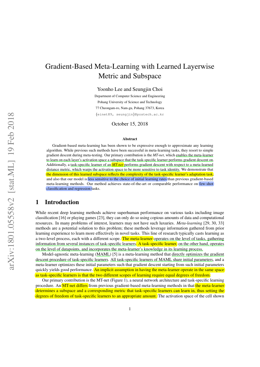
Our primary contribution is the MT-net (Figure 1), a neural network architecture and task-specific learning
procedure. An MT-net differs from previous gradient-based meta-learning methods in that the meta-learner
determines a subspace and a corresponding metric that task-specific learners can learn in, thus setting the
degrees of freedom of task-specific learners to an appropriate amount. The activation space of the cell shown
1
�
(a)
(b)
(c)
Figure 1: Task-specific learning in an MT-net. (a) A cell (rounded rectangle) consists of two layers. In addition
to initial weights (black), the meta-learner specifies weights to be changed (dotted lines) by task-specific
learners (colored). (b) Activation of this cell has 3 dimensions, but activation of task-specific learners only
change within a subspace (white plane). (c) The value of T affects task-specific learning so that gradients of
W are sensitive to task identity. Best seen in color.
in Figure 1 is 3-dimensional, but because the task-specific learners can only change weights that affect two of
the three intermediate activations, task-specific learning only happens on a subspace with 2 degrees of freedom.
Additionally, meta-learned parameters T alter the geometry of the activation space of task-specific parameters
so that task-specific learners are more sensitive to change in task.
2 Background
2.1 Problem Setup
We briefly explain the meta-learning problem setup which is applied to few-shot tasks.
The problems of k-shot regression and classification are as follows. In the training phase for a meta-learner,
we are given a (possibly infinite) set of tasks {T1,T2,T3, . . .}. Each task provides a training set and a test set
{DTi,train,DTi,test}. We assume here that the training set DTi,train has k examples per class, hence the name
k-shot learning. A particular task T ∈ {T1,T2,T3, . . .} is assumed to be drawn from the distribution of tasks
p(T ). Given a task T ∼ p(T ), the task-specific model fθT (a feedforward neural network is considered in this
Denote byθT parameters obtained by optimizing LT (θT ,DT ,train). Then, the meta-learner fθ is updated
paper) parameterized by θT is trained using the dataset DT ,train and its corresponding loss LT (θT ,DT ,train).
using the feedback from the collection of losses
, where the loss of each task
is evaluated using the test data DT ,test. Given a new task Tnew (not considered during meta-training), the
meta-learner helps the model fθTnew to quickly adapt to the new task Tnew, by warm-starting the gradient
updates.
T ∼p(T )
LT (θT ,DT ,test)
2.2 Model-Agnostic Meta-Learning
We briefly review model-agnostic meta-learning (MAML) [5], emphasizing commonalities and differences
between MAML and our method. MAML is a meta-learning method that applies to any model that learns
using gradient descent. This method is loosely inspired by fine-tuning, and it learns initial parameters of a
network such that the network’s loss after a few gradient steps is minimized.
2
�
Let us consider a model that is parameterized by θ. MAML alternates between the two updates (1) and (2)
to determine initial parameters θ for task-specific learners to warm-start the gradient descent updates, such that
new tasks can be solved using a small number of examples. Each task-specific learner updates its parameters
by the gradient update (1), using the loss evaluated with the data {DT ,train}. The meta-optimization across
tasks is performed such that the parameters θ are updated using the loss evaluated with {DT ,test}, which is
given in (2).
θT ← θ − α∇θLT (θ,DT ,train)
θ ← θ − β∇θ
T ∼p(T )
θT ,DT ,test
LT
,
(1)
(2)
where α > 0 and β > 0 are learning rates and the summation in (2) is computed using minibatches of tasks
sampled from p(T ).
Intuitively, a well-learned initial parameter θ is close to some local optimum for every task T ∼ p(T ).
Furthermore, the update (1) is sensitive to task identity in the sense thatθT1 andθT2 have different behaviors
for different tasks T1,T2 ∼ p(T ).
Recent work has shown that gradient-based optimization is a universal learning algorithm [4], in the sense
that any learning algorithm can be approximated up to arbitrary accuracy using some parameterized model and
gradient descent. Thus, no generality is lost by only considering gradient-based learners as in (1).
optimize performance after fine-tuning. However, while MAML updates all parameters in θ to makeθT , our
Our method is similar to MAML in that our method also differentiates through gradient update steps to
method only alters a (meta-learned) subset of its weights. Furthermore, whereas MAML learns with standard
gradient descent, a subset of our method’s parameters effectively ’warp’ the parameter space of the parameters
to be learned during meta-testing to enable faster learning.
3 Meta-Learning Models
We present our two models in this section: Transformation Networks (T-net) and Mask Transformation
Networks (MT-net), both of which are trained by gradient-based meta-learning. A T-net learns a metric in its
activation space; this metric informs each task-specific learner’s update direction and step size. An MT-net
additionally learns which subset of its weights to update for task-specific learning. Therefore, an MT-net learns
to automatically assign one of two roles (task-specific or task-mutual) to each of its weights.
3.1 T-net
We consider a model fθ(·), parameterized by θ. This model consists of L cells, where each cell is parameter-
ized∗ as TW:
fθ(x)
= TLWLσTL−1WL−1. . . σT1W1x ,
(3)
where x ∈ RD is an input, and σ(·) is a nonlinear activation function. T-nets get their name from transformation
matrices (T) because the linear transformation defined by a T plays a crucial role in meta-learning. Note that a
∗For convolutional cells, W is a convolutional layer with some size and stride and and T is a 1 × 1 convolution that doesn’t change
the number of channels
3
�
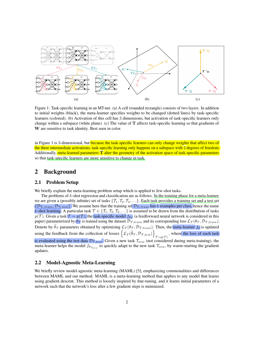
Figure 2: A diagram of the adaptation process of a Transformation Network (T-net). Blue values are meta-
learned and shared across all tasks. Orange values are different for each task.
cell has the same expressive power as a linear layer. Model parameters θ are a collection of W’s and T’s, i.e.,
W1, . . . , WL
θW
θT
θ =
, T1, . . . , TL
.
train set DT ,train. Thus we denote such (adjusted) parameters for task T asθW,T . Though they may look
Parameters θT, which are shared across task-specific models, are determined by the meta-learner. All task-
specific learners have the same initial θW but update to different values since each uses their corresponding
similar, T denotes tasks whereas T denotes a transformation matrix.
Given a task T sampled from p(T ), each W is adjusted with the gradient update
Again,θW,T is defined as {W1T , . . . ,WLT }. Using the task-specific learnerθW,T , the meta-learner improves
(4)
WT ← W − α∇WLT (θW, θT,DT ,train) .
.
θW,T , θT,DT ,test
LT
θ ← θ − β∇θ
T ∼p(T )
itself with the gradient update
α > 0 and β > 0 are learning rate hyperparameters. We show our full algorithm in Algorithm 1.
Suppose that we are given a new task T∗ with the training set DT∗,train. The model parametersθW,T∗
are computed as (4), where the gradient update starts from the initial value θW that was determined by the
meta-learner.
(5)
4
�
Sample batch of tasks Ti ∼ p(T )
for all Tj do
Algorithm 1 Transformation Networks (T-net)
Require: p(T )
Require: α, β
1: randomly initialize θ
2: while not done do
3:
4:
5:
6:
7:
8:
9:
10:
11: end while
ComputeWT according to (4)
θW,Tj = {W1Tj
,···WLTj
j LT (θW,Tj , θT,DTj ,test)
end for
θ ← θ − β∇θ
for i = 1,··· , L do
end for
}
We now briefly examine a single cell:
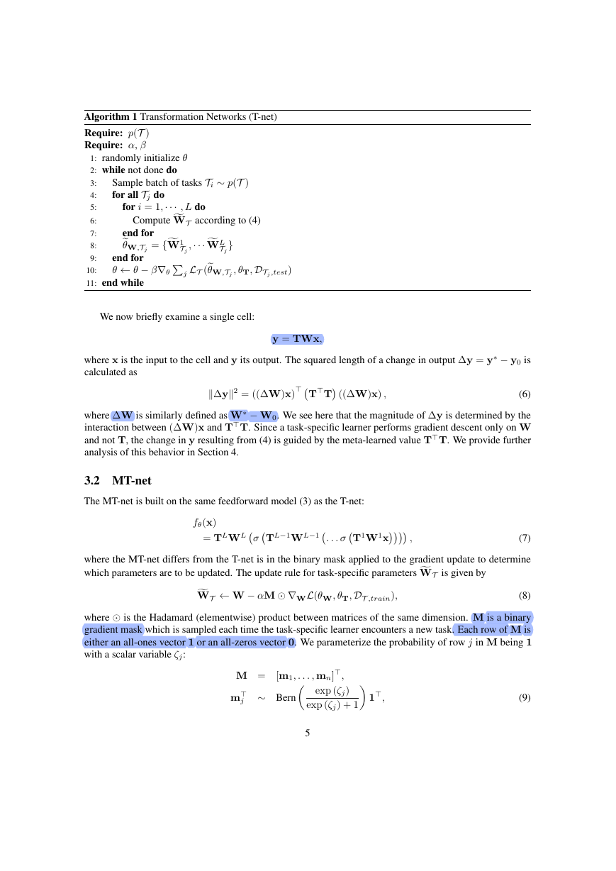
y = TWx,
where x is the input to the cell and y its output. The squared length of a change in output ∆y = y∗ − y0 is
calculated as
∆y2 = ((∆W)x)
(6)
where ∆W is similarly defined as W∗ − W0. We see here that the magnitude of ∆y is determined by the
interaction between (∆W)x and TT. Since a task-specific learner performs gradient descent only on W
and not T, the change in y resulting from (4) is guided by the meta-learned value TT. We provide further
analysis of this behavior in Section 4.
TT ((∆W)x) ,
3.2 MT-net
The MT-net is built on the same feedforward model (3) as the T-net:
fθ(x)
= TLWLσTL−1WL−1. . . σT1W1x ,
WT ← W − αM ∇WL(θW, θT,DT ,train),
where the MT-net differs from the T-net is in the binary mask applied to the gradient update to determine
which parameters are to be updated. The update rule for task-specific parametersWT is given by
(8)
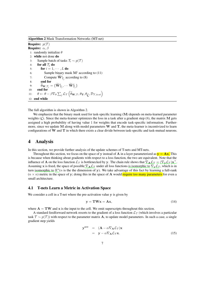
where is the Hadamard (elementwise) product between matrices of the same dimension. M is a binary
gradient mask which is sampled each time the task-specific learner encounters a new task. Each row of M is
either an all-ones vector 1 or an all-zeros vector 0. We parameterize the probability of row j in M being 1
with a scalar variable ζj:
(7)
M = [m1, . . . , mn],
j ∼ Bern
m
exp (ζj)
exp (ζj) + 1
5
1,
(9)
�
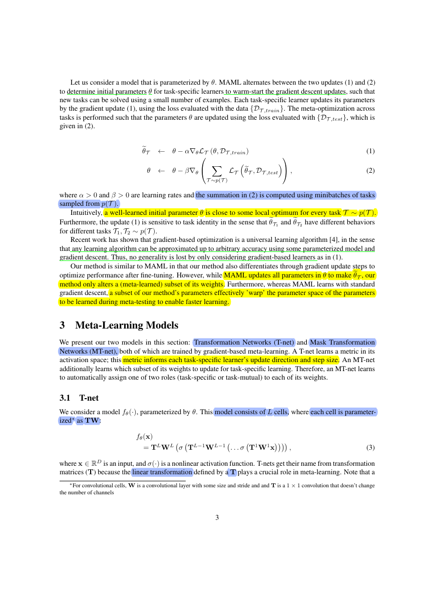
Figure 3: A diagram of the adaptation process of a Mask Transformation Network (MT-net). Blue values are
meta-learned and shared across all tasks. Orange values are different for each task.
where Bern(·) denotes the Bernoulli distribution. Each logit ζ acts on a row of a weight matrix W, so weights
that contribute to the same immediate activation are updated or not updated together.
We backpropagate through the Bernoulli sampling of masks using the Gumbel-Softmax estimator [12]:
g1, g2 ∼ Gumbel(0, 1),
j ←
m
exp
ζj +g1
+ exp g2
T
T
ζj +g1
exp
T
1,
(10)
(11)
where T is a temperature hyperparameter. This reparameterization allows us to directly backpropagate through
the mask, which at the limit of zero temperature, follows the behavior of (9).
As in T-nets, we denote the collection of altered weights asθW,T = {W1T , . . . ,WLT }. The meta-learner
learns all parameters θ:
θ =
, T1, . . . , TL
W1, . . . , WL
θW
T ∼p(T )
,
, ζ1, . . . , ζL
.
θW,T , θT, θζ ,DT ,test
.
θW,T , θT, θζ ,DT ,test
θζ
θT
:
(12)
(13)
θ ← θ − β∇θ
LT
As in a T-net, the meta-learner performs stochastic gradient descent on LT
6
�
Sample batch of tasks Ti ∼ p(T )
for all Tj do
for i = 1,··· , L do
Algorithm 2 Mask Transformation Networks (MT-net)
Require: p(T )
Require: α, β
1: randomly initialize θ
2: while not done do
3:
4:
5:
6:
7:
8:
9:
10:
11:
12: end while
ComputeWiTj
θW,Tj = {W1Tj
,···WLTj
θW,T , θT, θζ ,DT ,test
j LT
Sample binary mask Mi according to (11)
end for
end for
θ ← θ − β∇θ
according to (8)
}
The full algorithm is shown in Algorithm 2.
We emphasize that the binary mask used for task-specific learning (M) depends on meta-learned parameter
weights (ζ). Since the meta-learner optimizes the loss in a task after a gradient step (8), the matrix M gets
assigned a high probability of having value 1 for weights that encode task-specific information. Further-
more, since we update M along with model parameters W and T, the meta-learner is incentivized to learn
configurations of W and T in which there exists a clear divide between task-specific and task-mutual neurons.
4 Analysis
In this section, we provide further analysis of the update schemes of T-nets and MT-nets.
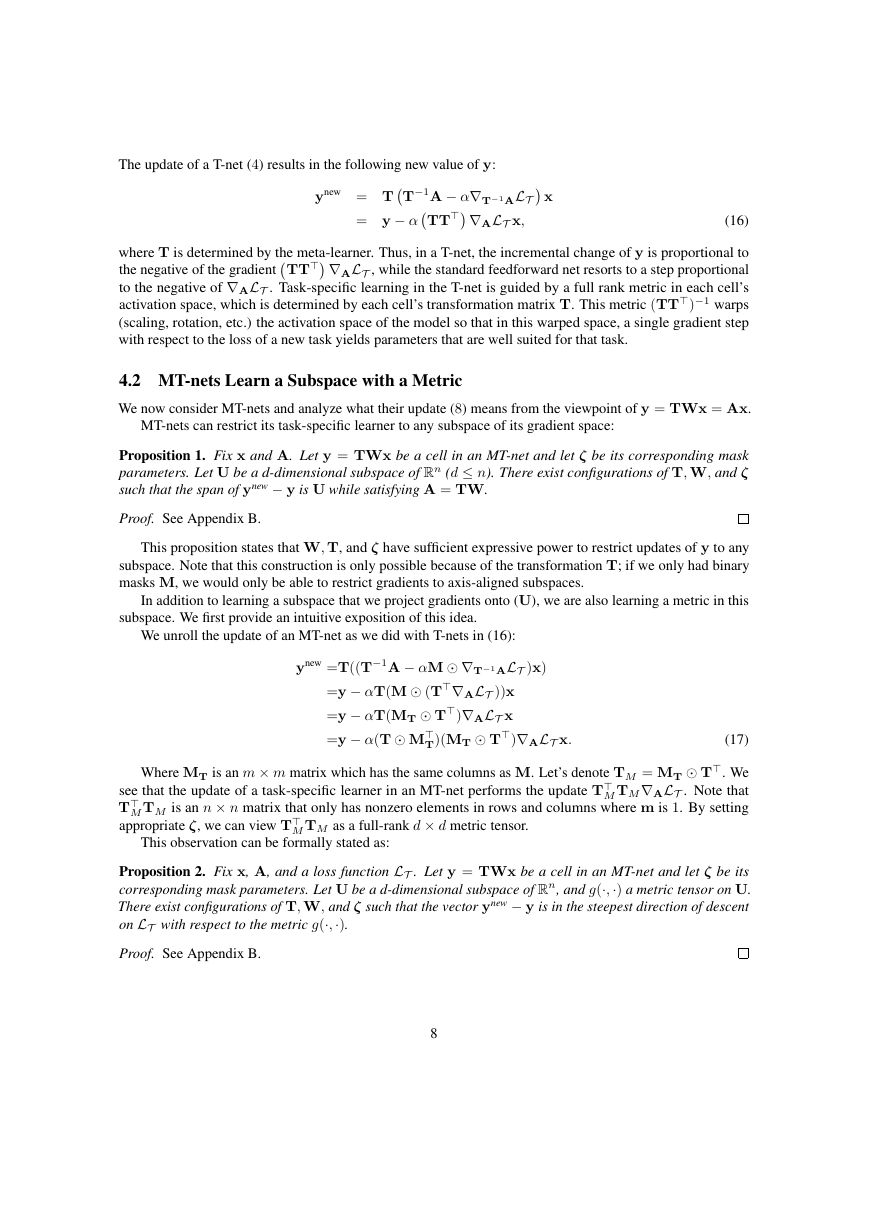
Throughout this section, we focus on the space of y instead of A in a layer parameterized as y = Ax. This
is because when thinking about gradients with respect to a loss function, the two are equivalent. Note that the
influence of A on the loss function LT is bottlenecked by y. The chain rule shows that ∇ALT = (∇yLT )x.
Assuming x is fixed, the space of possible ∇ALT under all loss functions is isomorphic to ∇yLT , which is in
turn isomorphic to Rn(n is the the dimension of y). We take advantage of this fact by learning a full-rank
(n × n) metric in the space of y; doing this in the space of A would require too many parameters for even a
small architecture.
4.1 T-nets Learn a Metric in Activation Space
We consider a cell in a T-net where the pre-activation value y is given by
y = TWx = Ax,
(14)
where A = TW and x is the input to the cell. We omit superscripts throughout this section.
A standard feedforward network resorts to the gradient of a loss function LT (which involves a particular
task T ∼ p(T )) with respect to the parameter matrix A, to update model parameters. In such a case, a single
gradient step yields
ynew = (A − α∇ALT )x
= y − α∇ALT x.
7
(15)
�
The update of a T-net (4) results in the following new value of y:
ynew = TT−1A − α∇T−1ALT x
= y − αTT∇ALT x,
the negative of the gradientTT∇ALT , while the standard feedforward net resorts to a step proportional
where T is determined by the meta-learner. Thus, in a T-net, the incremental change of y is proportional to
to the negative of ∇ALT . Task-specific learning in the T-net is guided by a full rank metric in each cell’s
activation space, which is determined by each cell’s transformation matrix T. This metric (TT)−1 warps
(scaling, rotation, etc.) the activation space of the model so that in this warped space, a single gradient step
with respect to the loss of a new task yields parameters that are well suited for that task.
(16)
4.2 MT-nets Learn a Subspace with a Metric
We now consider MT-nets and analyze what their update (8) means from the viewpoint of y = TWx = Ax.
MT-nets can restrict its task-specific learner to any subspace of its gradient space:
Proposition 1. Fix x and A. Let y = TWx be a cell in an MT-net and let ζ be its corresponding mask
parameters. Let U be a d-dimensional subspace of Rn (d ≤ n). There exist configurations of T, W, and ζ
such that the span of ynew − y is U while satisfying A = TW.
Proof. See Appendix B.
This proposition states that W, T, and ζ have sufficient expressive power to restrict updates of y to any
subspace. Note that this construction is only possible because of the transformation T; if we only had binary
masks M, we would only be able to restrict gradients to axis-aligned subspaces.
In addition to learning a subspace that we project gradients onto (U), we are also learning a metric in this
subspace. We first provide an intuitive exposition of this idea.
We unroll the update of an MT-net as we did with T-nets in (16):
ynew =T((T−1A − αM ∇T−1ALT )x)
=y − αT(M (T∇ALT ))x
=y − αT(MT T)∇ALT x
=y − α(T M
T)(MT T)∇ALT x.
(17)
Where MT is an m × m matrix which has the same columns as M. Let’s denote TM = MT T. We
M TM∇ALT . Note that
see that the update of a task-specific learner in an MT-net performs the update T
M TM is an n × n matrix that only has nonzero elements in rows and columns where m is 1. By setting
T
appropriate ζ, we can view T
M TM as a full-rank d × d metric tensor.
This observation can be formally stated as:
Proposition 2. Fix x, A, and a loss function LT . Let y = TWx be a cell in an MT-net and let ζ be its
corresponding mask parameters. Let U be a d-dimensional subspace of Rn, and g(·,·) a metric tensor on U.
There exist configurations of T, W, and ζ such that the vector ynew − y is in the steepest direction of descent
on LT with respect to the metric g(·,·).
Proof. See Appendix B.
8
�



 2023年江西萍乡中考道德与法治真题及答案.doc
 2012年重庆南川中考生物真题及答案.doc
 2013年江西师范大学地理学综合及文艺理论基础考研真题.doc
 2020年四川甘孜小升初语文真题及答案I卷.doc
 2020年注册岩土工程师专业基础考试真题及答案.doc
 2023-2024学年福建省厦门市九年级上学期数学月考试题及答案.doc
 2021-2022学年辽宁省沈阳市大东区九年级上学期语文期末试题及答案.doc
 2022-2023学年北京东城区初三第一学期物理期末试卷及答案.doc
 2018上半年江西教师资格初中地理学科知识与教学能力真题及答案.doc
 2012年河北国家公务员申论考试真题及答案-省级.doc
 2020-2021学年江苏省扬州市江都区邵樊片九年级上学期数学第一次质量检测试题及答案.doc
 2022下半年黑龙江教师资格证中学综合素质真题及答案.doc