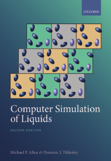
Cover
Preface
Contents
1 Introduction
1.1 A short history of computer simulation
1.2 Computer simulation: motivation and applications
1.3 Model systems and interaction potentials
1.4 Constructing an intermolecular potential from first principles
1.5 Force fields
1.6 Studying small systems
2 Statistical mechanics
2.1 Sampling from ensembles
2.2 Common statistical ensembles
2.3 Transforming between ensembles
2.4 Simple thermodynamic averages
2.5 Fluctuations
2.6 Structural quantities
2.7 Time correlation functions and transport coefficients
2.8 Long-range corrections
2.9 Quantum corrections
2.10 Constraints
2.11 Landau free energy
2.12 Inhomogeneous systems
2.13 Fluid membranes
2.14 Liquid crystals
3 Molecular dynamics
3.1 Equations of motion for atomic systems
3.2 Finite-difference methods
3.3 Molecular dynamics of rigid non-spherical bodies
3.4 Constraint dynamics
3.5 Multiple-timestep algorithms
3.6 Checks on accuracy
3.7 Molecular dynamics of hard particles
3.8 Constant-temperature molecular dynamics
3.9 Constant-pressure molecular dynamics
3.10 Grand canonical molecular dynamics
3.11 Molecular dynamics of polarizable systems
4 Monte Carlo methods
4.1 Introduction
4.2 Monte Carlo integration
4.3 Importance sampling
4.4 The Metropolis method
4.5 Isothermal–isobaric Monte Carlo
4.6 Grand canonical Monte Carlo
4.7 Semi-grand Monte Carlo
4.8 Molecular liquids
4.9 Parallel tempering
4.10 Other ensembles
5 Some tricks of the trade
5.1 Introduction
5.2 The heart of the matter
5.3 Neighbour lists
5.4 Non-bonded interactions and multiple timesteps
5.5 When the dust has settled
5.6 Starting up
5.7 Organization of the simulation
5.8 Checks on self-consistency
6 Long-range forces
6.1 Introduction
6.2 The Ewald sum
6.3 The particle–particle particle–mesh method
6.4 Spherical truncation
6.5 Reaction field
6.6 Fast multipole methods
6.7 The multilevel summation method
6.8 Maxwell equation molecular dynamics
6.9 Long-range potentials in slab geometry
6.10 Which scheme to use?
7 Parallel simulation
7.1 Introduction
7.2 Parallel loops
7.3 Parallel replica exchange
7.4 Parallel domain decomposition
7.5 Parallel constraints
8 How to analyse the results
8.1 Introduction
8.2 Liquid structure
8.3 Time correlation functions
8.4 Estimating errors
8.5 Correcting the results
9 Advanced Monte Carlo methods
9.1 Introduction
9.2 Estimation of the free energy
9.3 Smarter Monte Carlo
9.4 Simulation of phase equilibria
9.5 Reactive Monte Carlo
10 Rare event simulation
10.1 Introduction
10.2 Transition state approximation
10.3 Bennett–Chandler approach
10.4 Identifying reaction coordinates and paths
10.5 Transition path sampling
10.6 Forward flux and transition interface sampling
10.7 Conclusions
11 Nonequilibrium molecular dynamics
11.1 Introduction
11.2 Spatially oscillating perturbations
11.3 Spatially homogeneous perturbations
11.4 Inhomogeneous systems
11.5 Flow in confined geometry
11.6 Nonequilibrium free-energy measurements
11.7 Practical points
11.8 Conclusions
12 Mesoscale methods
12.1 Introduction
12.2 Langevin and Brownian dynamics
12.3 Brownian dynamics, molecular dynamics, and Monte Carlo
12.4 Dissipative particle dynamics
12.5 Multiparticle collision dynamics
12.6 The lattice-Boltzmann method
12.7 Developing coarse-grained potentials
13 Quantum simulations
13.1 Introduction
13.2 Ab-initio molecular dynamics
13.3 Combining quantum and classical force-field simulations
13.4 Path-integral simulations
13.5 Quantum random walk simulations
13.6 Over our horizon
14 Inhomogeneous fluids
14.1 The planar gas–liquid interface
14.2 The gas–liquid interface of a molecular fluid
14.3 The liquid–liquid interface
14.4 The solid–liquid interface
14.5 The liquid drop
14.6 Fluid membranes
14.7 Liquid crystals
Appendix A Computers and computer simulation
A.1 Computer hardware
A.2 Programming languages
A.3 Fortran programming considerations
Appendix B Reduced units
B.1 Reduced units
Appendix C Calculation of forces and torques
C.1 Introduction
C.2 The polymer chain
C.3 The molecular fluid with multipoles
C.4 The triple-dipole potential
C.5 Charged particles using Ewald sum
C.6 The Gay–Berne potential
C.7 Numerically testing forces and torques
Appendix D Fourier transforms and series
D.1 The Fourier transform
D.2 Spatial Fourier transforms and series
D.3 The discrete Fourier transform
D.4 Numerical Fourier transforms
Appendix E Random numbers
E.1 Random number generators
E.2 Uniformly distributed random numbers
E.3 Generating non-uniform distributions
E.4 Random vectors on the surface of a sphere
E.5 Choosing randomly and uniformly from complicated regions
E.6 Generating a random permutation
Appendix F Configurational temperature
F.1 Expression for configurational temperature
F.2 Implementation details
List of Acronyms
List of Greek Symbols
List of Roman Symbols
List of Examples
List of Codes
Bibliography
Index





 2023年江西萍乡中考道德与法治真题及答案.doc
 2012年重庆南川中考生物真题及答案.doc
 2013年江西师范大学地理学综合及文艺理论基础考研真题.doc
 2020年四川甘孜小升初语文真题及答案I卷.doc
 2020年注册岩土工程师专业基础考试真题及答案.doc
 2023-2024学年福建省厦门市九年级上学期数学月考试题及答案.doc
 2021-2022学年辽宁省沈阳市大东区九年级上学期语文期末试题及答案.doc
 2022-2023学年北京东城区初三第一学期物理期末试卷及答案.doc
 2018上半年江西教师资格初中地理学科知识与教学能力真题及答案.doc
 2012年河北国家公务员申论考试真题及答案-省级.doc
 2020-2021学年江苏省扬州市江都区邵樊片九年级上学期数学第一次质量检测试题及答案.doc
 2022下半年黑龙江教师资格证中学综合素质真题及答案.doc