Briefing of mass load caused site displacements On seasonal time scales, surface mass load caused seasonal site displacements are the main feature of the space geodesy observed site position time series (see Dong et al. 2002). In many applications, space geodesy (like GPS) observed seasonal site displacements become important signals to compare with mass loading predicted seasonal site displacements due to various geophysical processes. In this case, mass loading caused site displacements should be calculated explicitly from independent geophysical data. QOCA utility mload provides such a function to calculate the site displacements from atmospheric pressure, pole tide, non-tidal ocean mass, snow and soil moisture. The mload adopts the Green's function approach to calculate the mass load caused site displacements. All the Green's functions are defined in the CE frame (center of mass of the solid Earth). The space geodesy solutions are usually aligned to the ITRF frame. The origin of the ITRF frame is officially defined as the CM frame (center of mass of the whole Earth including atmosphere and oceans). If that is true, the mass load predicted seasonal site displacements cannot be compared directly with the space geodesy observed seasonal site dislacements due to the inconsistency of the reference frames (CE vs. CM). However, on the seasonal time scales, the realized nature of the ITRF origin is not the CM, but the CF (center of the surface figure of the Earth) (see details in Dong et al. 2003). Since the difference between CE and CF is very small, so that in practice we can compare the solutions between the mass load predicted and the space geodesy observed site displacements. To run the mload, just typing: mload mload.drv All the commands are stored in the mload.drv file. The mload.drv file has the same structure and convention as other QOCA driver file. If you are not familiar with the driver file, please look at the basic class web page first. 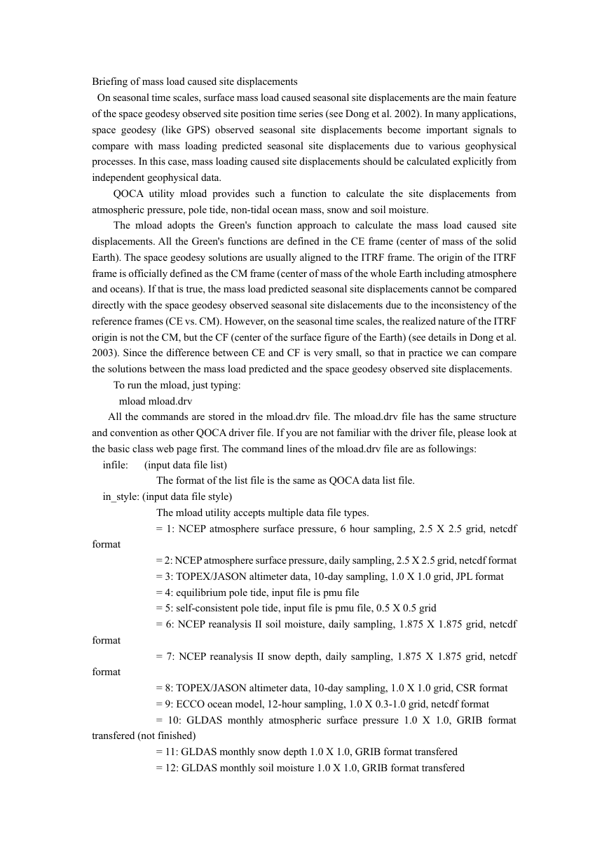The command lines of the mload.drv file are as followings: infile: (input data file list) The format of the list file is the same as QOCA data list file. in_style: (input data file style) The mload utility accepts multiple data file types. = 1: NCEP atmosphere surface pressure, 6 hour sampling, 2.5 X 2.5 grid, netcdf format = 2: NCEP atmosphere surface pressure, daily sampling, 2.5 X 2.5 grid, netcdf format = 3: TOPEX/JASON altimeter data, 10-day sampling, 1.0 X 1.0 grid, JPL format = 4: equilibrium pole tide, input file is pmu file = 5: self-consistent pole tide, input file is pmu file, 0.5 X 0.5 grid = 6: NCEP reanalysis II soil moisture, daily sampling, 1.875 X 1.875 grid, netcdf format = 7: NCEP reanalysis II snow depth, daily sampling, 1.875 X 1.875 grid, netcdf format = 8: TOPEX/JASON altimeter data, 10-day sampling, 1.0 X 1.0 grid, CSR format = 9: ECCO ocean model, 12-hour sampling, 1.0 X 0.3-1.0 grid, netcdf format = 10: GLDAS monthly atmospheric surface pressure 1.0 X 1.0, GRIB format transfered (not finished) = 11: GLDAS monthly snow depth 1.0 X 1.0, GRIB format transfered = 12: GLDAS monthly soil moisture 1.0 X 1.0, GRIB format transfered 

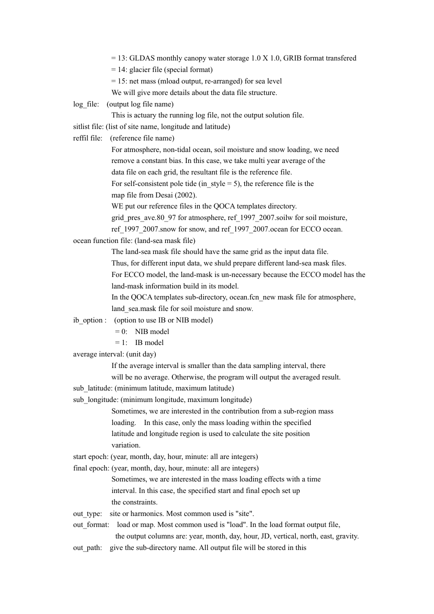
= 13: GLDAS monthly canopy water storage 1.0 X 1.0, GRIB format transfered = 14: glacier file (special format) = 15: net mass (mload output, re-arranged) for sea level We will give more details about the data file structure. log_file: (output log file name) This is actuary the running log file, not the output solution file. sitlist file: (list of site name, longitude and latitude) reffil file: (reference file name) For atmosphere, non-tidal ocean, soil moisture and snow loading, we need remove a constant bias. In this case, we take multi year average of the data file on each grid, the resultant file is the reference file. For self-consistent pole tide (in_style = 5), the reference file is the map file from Desai (2002). WE put our reference files in the QOCA templates directory. grid_pres_ave.80_97 for atmosphere, ref_1997_2007.soilw for soil moisture, ref_1997_2007.snow for snow, and ref_1997_2007.ocean for ECCO ocean. ocean function file: (land-sea mask file) The land-sea mask file should have the same grid as the input data file. Thus, for different input data, we shuld prepare different land-sea mask files. For ECCO model, the land-mask is un-necessary because the ECCO model has the land-mask information build in its model. In the QOCA templates sub-directory, ocean.fcn_new mask file for atmosphere, land_sea.mask file for soil moisture and snow. ib_option : (option to use IB or NIB model) = 0: NIB model = 1: IB model average interval: (unit day) If the average interval is smaller than the data sampling interval, there will be no average. Otherwise, the program will output the averaged result. sub_latitude: (minimum latitude, maximum latitude) sub_longitude: (minimum longitude, maximum longitude) Sometimes, we are interested in the contribution from a sub-region mass loading. In this case, only the mass loading within the specified latitude and longitude region is used to calculate the site position variation. start epoch: (year, month, day, hour, minute: all are integers) final epoch: (year, month, day, hour, minute: all are integers) Sometimes, we are interested in the mass loading effects with a time interval. In this case, the specified start and final epoch set up the constraints. out_type: site or harmonics. Most common used is "site". out_format: load or map. Most common used is "load". In the load format output file, the output columns are: year, month, day, hour, JD, vertical, north, east, gravity. out_path: give the sub-directory name. All output file will be stored in this 

sub-directory. Atmospheric mass loading calculation In mload, we use NCEP reanalysis atmospheric surface pressure data to calculate mass loading caused site displacemnts. NCEP uses NetCDF format to archive their reanalysis solutions. Our mload program enbeds a simplified tool to read the NetCDF format file. More general reading tool requires the installations of both netcdf and udunit libraries. NetCDF (network Common Data Form) is an interface for array-oriented data access and a library that provides an implementation of the interface. The netCDF library also defines a machine- independent format for representing scientific data. Together, the interface, library, and format support the creation, access, and sharing of scientific data. In NetCDF file, the data is divided into several parts. The reading tool restores the final data by the formula: final_data = read_data * scale + offset The unit of NCEP reanalysis atmosphere surface pressure data is Pascal. Since we are interested in the variations of the surface pressure caused site displacements, not the absolute displacements, we subtract a reference value at each grid. In mload, such a reference values are obtaines in a reference file. For atmospheric mass loading, the reference file is derived by multi-year average of the surface pressure data on each grid. The site displacements from the global surface pressure data are calculated using Green's function approach. In mload, we use Farrel's Green functions. For the ocean's response to surface pressure variations, the "Inverted Barometer" (IB) model is generally adopted. Such an IB assumption is probably valid for low frequency variations (period more than one day). For high- frequency variations, the ocean's fluid dynamics might be taken into account. In mload.drv file, the option of choosing IB or NIB model is realized by the "ib_option" command line. The mload program recognizes two types of NCEP reanalysis surface pressure data files: 6-hour sampling and 1-day average files. Sometimes, we only need averaged results, for example the daily- mean site displacements rather than 6-hour site displacements. The mload program has an option "average interval" to realize the average. If you specify 1.0, mload will output daily mean site displacements. If you specify 5.0, mload will output 5-day mean site displacements. The mload program also provides the option to specify region (box region bounded by latitude and longitude) and time interval (start and end epochs). These options bring flexibility to perform more detailed research. The "outfile" in mload.drv is not the output solution file. It actuary is a log file, which records some running and data i/o information. The output solution files are site_name.aload. Here the site_name is from the "sitlist" file. If there are multiple sites in the "sitlist" file, the mload will output multiple output solution files. Here the suffix "aload" of the output file name is fixed for mload, which represents the site displacements caused by atmosphere loading. 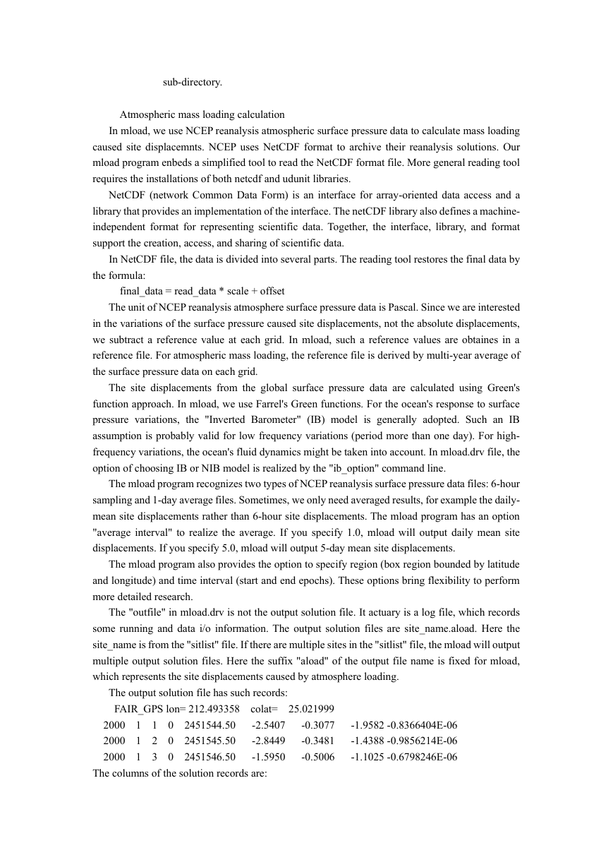The output solution file has such records: FAIR_GPS lon= 212.493358 colat= 25.021999 2000 1 1 0 2451544.50 -2.5407 -0.3077 -1.9582 -0.8366404E-06 2000 1 2 0 2451545.50 -2.8449 -0.3481 -1.4388 -0.9856214E-06 2000 1 3 0 2451546.50 -1.5950 -0.5006 -1.1025 -0.6798246E-06 The columns of the solution records are: 

year month day hour JD vertical north east gravity Where the unit of the site displacements is mm (positive in up, north, east directions). Please click the selection button of the above window to see the various file formats. Since the NCEP reanalysis surface presure data file uses the 2.5 X 2.5 grid, the ocean function file should use the same 2.5 X 2.5 resolution land-sea mask file, where the value great than 0 means land, others are ocean. Non-tidal ocean mass loading We use the TOPEX/Posaidon, JASON altimeter measurements as the input data. These data directly measure the sea surface height. Since there are many contributors affect the sea surface height, the relatively well-known (or can be easily modeled) contributions are modeled and removed from the final result. Soil moisture mass loading Snow mass loading GLDAS model GLDAS (Global Land Data Assimilation System) is a modern land surface state and flux assimilation system. It is based on the land surface models and integrates huge observation data to generate the products. Currently it has 4 commonly used models: Mosaic, Noah, CLM (Community Land Model) and VIC (Variable Infiltration Capacity) models. Its temporal resolution is 3-hourly. Monthly products are generated through averaging the 3-hourly products. Currently, mload is mainly focused on the NOAH (NCEP, Oregon State University, United States Air Force, and Office of Hydrology) model, which has 1 x 1 and 0.25 x 0.25 spatial resolution solutions. Currently only 1 x 1 model is well tested. Note the GLDAS model covers only latitude 60S to 90N region, so that the surface mass redistribution in Antarctica must be calculated using other data sets. Since the observational constrains in Greenland are poor, the GLDAS solutions in Greenland are not very reliable. GLDAS files are in GRIB format and include all surface state solutions. To save the analysis time, MLOAD accepts only reorganized text format. To generate the MLOAD recognized format file, please use the following wgrib commands. 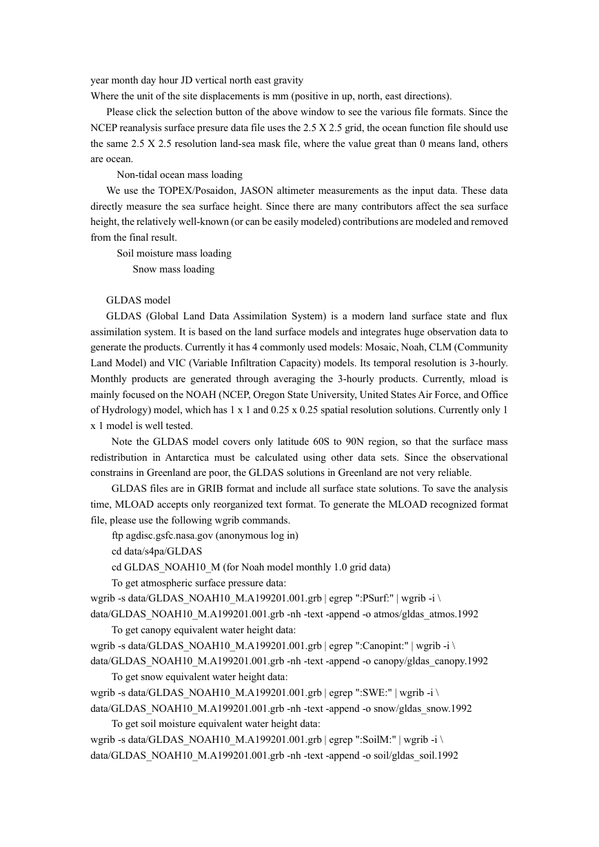ftp agdisc.gsfc.nasa.gov (anonymous log in) cd data/s4pa/GLDAS cd GLDAS_NOAH10_M (for Noah model monthly 1.0 grid data) To get atmospheric surface pressure data: wgrib -s data/GLDAS_NOAH10_M.A199201.001.grb | egrep ":PSurf:" | wgrib -i \ data/GLDAS_NOAH10_M.A199201.001.grb -nh -text -append -o atmos/gldas_atmos.1992 To get canopy equivalent water height data: wgrib -s data/GLDAS_NOAH10_M.A199201.001.grb | egrep ":Canopint:" | wgrib -i \ data/GLDAS_NOAH10_M.A199201.001.grb -nh -text -append -o canopy/gldas_canopy.1992 To get snow equivalent water height data: wgrib -s data/GLDAS_NOAH10_M.A199201.001.grb | egrep ":SWE:" | wgrib -i \ data/GLDAS_NOAH10_M.A199201.001.grb -nh -text -append -o snow/gldas_snow.1992 To get soil moisture equivalent water height data: wgrib -s data/GLDAS_NOAH10_M.A199201.001.grb | egrep ":SoilM:" | wgrib -i \ data/GLDAS_NOAH10_M.A199201.001.grb -nh -text -append -o soil/gldas_soil.1992 

In mload driver file, when you specify the correct in_style, mload can analyzes these GLDAS transferred files. Note for the soil moisture different models have different layer number. For example, CLS model has 10 layers and Noah model has 4 layers. In this case, users should specify the layer number to distinquish different models. For example, if user wants to process Noah model soil moisture data file, the command is: in_style : 12 4 The last number represents the layer number. Currently mload implements the "exclude" option for GLDAS format (in_style 12, 13, 14). To execise this option, the driver file should add this command line: exclude region file : exclu.region The format of the exclu.region is as followings: 2 0.0 359.0 -90.0 -60.0 # Antarctica 290.0 345.0 62.0 85.0 # Greenland + small part of Canada ---- NOT FINISHED YET ----