Journal of Geoscience and Environment Protection, 2017, 5, 183-197
http://www.scirp.org/journal/gep
ISSN Online: 2327-4344
ISSN Print: 2327-4336
Geographical Analysis of Lung Cancer Mortality
Rate and PM2.5 Using Global Annual Average
PM2.5 Grids from MODIS and MISR Aerosol
Optical Depth
Zhiyong Hu*, Ethan Baker
Department of Earth & Environmental Studies, University of West Florida, Pensacola, USA
How to cite this paper: Hu, Z.Y. and Bak-
er, E. (2017) Geographical Analysis of Lung
Cancer Mortality Rate and PM2.5 Using
Global Annual Average PM2.5 Grids from
MODIS and MISR Aerosol Optical Depth.
Journal of Geoscience and Environment
Protection, 5, 183-197.
https://doi.org/10.4236/gep.2017.56017
Received: May 23, 2017
Accepted: June 27, 2017
Published: June 30, 2017
Abstract
Exposure to particulate matter with an aerodynamic diameter of less than 2.5
μm (PM2.5) may increase risk of lung cancer. The repetitive and broad-area
coverage of satellites may allow atmospheric remote sensing to offer a unique
opportunity to monitor air quality and help fill air pollution data gaps that
hinder efforts to study air pollution and protect public health. This geograph-
ical study explores if there is an association between PM2.5 and lung cancer
mortality rate in the conterminous USA. Lung cancer (ICD-10 codes C34-
C34) death count and population at risk by county were extracted for the pe-
riod from 2001 to 2010 from the U.S. CDC WONDER online database. The
2001-2010 Global Annual Average PM2.5 Grids from MODIS and MISR Aero-
sol Optical Depth dataset was used to calculate a 10 year average PM2.5 pollu-
tion. Exploratory spatial data analyses, spatial regression (a spatial lag and a
spatial error model), and spatially extended Bayesian Monte Carlo Markov
Chain simulation found that there is a significant positive association between
lung cancer mortality rate and PM2.5. The association would justify the need of
further toxicological investigation of the biological mechanism of the adverse
effect of the PM2.5 pollution on lung cancer. The Global Annual Average PM2.5
Grids from MODIS and MISR Aerosol Optical Depth dataset provides a con-
tinuous surface of concentrations of PM2.5 and is a useful data source for en-
vironmental health research.
Keywords
Lung Cancer, PM2.5, Remote Sensing, GIS, Exploratory Spatial Data Analysis,
Spatial Regression, Bayesian MCMC Simulation
DOI: 10.4236/gep.2017.56017 June 30, 2017
�
Z. Y. Hu, E. Baker
184
1. Introduction
Lung cancer is a leading cause of cancer mortality in the United States. Exposure
to particulate matter with an aerodynamic diameter of less than 2.5 μm (PM2.5)
may increase risk of lung cancer [5]. The World Health Organization (WHO)
guideline for PM2.5 average annual exposure is less than or equal to 10.0 μg/m3,
and the US Environmental Protection Agency (EPA) sets an annual average
PM2.5 standard of 12 μg/m3. Recently findings on air pollution and lung cancer
incidence in 17 European cohorts show that long term exposure to particulate
air pollution increases the risk of lung cancer, even at levels below the European
Union limit value (25 μg/m3) (Raaschou-Nielsen et al. 2013).
Air pollution (including PM2.5) epidemiological studies often rely on ground
monitoring networks to provide metrics of exposure. Ground monitoring data
often lacks spatially complete coverage. Public health concerns compel efforts to
broaden spatial and temporal coverage. The repetitive and broad-area coverage
of satellites may allow atmospheric remote sensing to offer a unique opportunity
to monitor air quality at continental, national and regional scales. To provide a
continuous surface of concentrations of PM2.5 for health and environmental re-
search, researchers at Battelle Memorial Institute in collaboration with the Cen-
ter for International Earth Science Information Network/Columbia University
have developed Global Annual Average PM2.5 Grids from MODIS and MISR
Aerosol Optical Depth (AOD) covering year 2001 to 2010 [3]. There are few stu-
dies using this dataset to assess PM2.5 effect on lung cancer.
This study was to examine if there is an association between PM2.5 and lung
cancer mortality rate in the conterminous USA using the Global Annual Average
PM2.5 Grids. The study used a suite of geographical approach, including remote
sensing, GIS, cartography (map visualization and comparison), exploratory spa-
tial data analysis (ESDA) and spatially extended statistical models.
2. Methods
2.1. PM2.5 Data
The 2001-2010 Global Annual Average PM2.5 Grids from Moderate Resolution
Imaging Spectroradiometer (MODIS) and Multi-angle Imaging Spectroradi-
ometer (MISR) Aerosol Optical Depth (AOD) dataset [3] were used to calculate
a global 10-year (2001-2010) average PM2.5 grid. This global grid was then
clipped to the study area—the conterminous USA.
In the Global Annual Average PM2.5 Grids data archive, each annual average
data file contains integer values for a global grid (0.5˚ × 0.5˚) of estimated PM2.5
concentrations (in µg/m3) covering the world from 70˚N to 60˚S.The MODIS
and MISR AOD retrievals were converted to ground-level concentrations based
on a conversion factor developed by van Donkelaar et al. (2010). Level 3 global,
monthly-mean MODIS and MISR AOD data for the years 2001-2010 were ac-
quired from NASA LAADS and NASA Langley ASDC respectively. The MODIS
level 3 (L3) monthly data were disaggregated from 1˚ resolution to 0.5˚ resolu-
�
Z. Y. Hu, E. Baker
tion to match the resolution of the MISR AOD data. AOD for both instruments
that were anticipated to have a bias of greater than ±(0.1 uhuior 20%) as com-
pared to ground-based Aerosol Robotic Network (AERONET; Holben et al.
1998) AOD due to high surface albedos or other persistent factors were removed
from the analysis. The filtered MODIS and MISR data were then combined by
taking the mean of each grid cell for each month of the year. Ground-level con-
centrations of dry 24 hour PM2.5 were estimated from the satellite observations
of total-column AOD by applying a conversion factor that accounts for the spa-
tial and temporal relationship between the two. This conversion factor is a func-
tion of aerosol size, aerosol type, diurnal variation, relative humidity and the
vertical structure of aerosol extinction, which were derived from a global 3-D
chemical transport model (GEOS-Chem: http://acmg.seas.harvard.edu/geos/)
and assumes a relative humidity of 50% (van Donkelaar et al. 2010). The satellite
AOD data were multiplied by monthly-mean conversion factors (calculated as a
climatological mean over 2001-2006) for each grid cell. Finally, an annual-aver-
age estimated surface PM2.5 concentration was estimated by calculating the
mean of the monthly estimates over each year.
2.2. Lung Cancer Data
Lung cancer (ICD-10 codes C34-C34: malignant neoplasms of trachea, bronchus
and lung) death count and population at risk by county for the conterminous
USA were extracted for the period from 2001 to 2010 from the National Center
for Health Statistics Compressed Mortality File 1999-2010 in the CDC
WONDER online database [4]. Age adjusted rate was calculated using direct
standardization for each county. The year 2000 US decennial census data was
used as a standard population to standardize rates. Expected count of lung can-
cer was also calculated which is the number of cases that would be expected in
the study population if people in the study population contracted the disease at
the same rate as people in the standard population. Age-adjusted death rates are
weighted averages of the age-specific death rates, where the weights represent a
fixed population by age. They are used to compare relative mortality risk among
groups and over time. An age-adjusted rate represents the rate that would have
existed had the age-specific rates of the particular year prevailed in a population
whose age distribution was the same as that of the fixed population. Age adjust-
ment is a technique for removing the effects of age from crude rates, so as to al-
low meaningful comparisons across populations with different underlying age
structures. Age-adjusted rates should be viewed as relative indexes rather than as
direct or actual measures of mortality risk. According to Curtin and Klein [6],
one of the problems with rate adjustment is that rates based on small numbers of
deaths will exhibit a large amount of random variation. In the lung cancer mor-
tality count and population data set, crude death rates and age-adjusted death
rates are marked as “unreliable” when the death count is less than 20. Lung
death counts are “suppressed” when the data meets the criteria for confidential-
ity constraints. Sub-national data representing fewer than ten persons are sup-
185
�
Z. Y. Hu, E. Baker
186
pressed. All counties with unreliable and suppressed data were not included in
the following spatial analyses. After excluding counties that have unreliable or
suppressed data, the number of data points (counties) for the analysis is 2,931.
2.3. Exploratory Spatial Data Analysis
To link lung cancer mortality rate with PM2.5, the 10-year (2001-2010) mean
PM2.5 raster grid was first resampled so that each 0.5˚ × 0.5˚ grid cell was subdi-
vided into 20 by 20 smaller cells retaining the original PM2.5 values. The purpose
of the resampling procedure was to split the grid cell on the county boundary
into smaller cells for neighboring counties to achieve higher accuracy of county
average PM2.5 calculation.
The resampled PM2.5 grid was then overlaid with the map of lung cancer mor-
tality rates. A GIS zonal statistical function was used to calculate the average
PM2.5 value for each county. The average value was calculated by averaging PM2.5
values of all the cells formed after the resampling of the original grid whose cen-
troids are within the county.
Exploratory spatial data analysis (ESDA) [1] methods were used to examine
the spatial autocorrelation within the spatial data and explore the association
between lung cancer mortality rate and PM2.5. The analysis involved calculation
of univariate global Moran’s I statistic and local indicator of spatial association
(LISA) [2]. Spatial contiguity was assessed as Queen’s contiguity which defines
spatial neighbors as those areas with shared borders and vertexes. Univariate
global Moran’s I examines the degree of spatial autocorrelation in the mortality
rate and PM2.5 maps respectively. LISA provides information relating to the loca-
tion of spatial clusters and outliers and the types of spatial correlation. Local sta-
tistics are important because the magnitude of spatial autocorrelation is not
necessarily uniform over the study area [1].
Univariate LISA resulted in a cluster map for each of the two variables. Biva-
riate LISA results were presented as a Moran scatter plot and a cluster map. Bi-
variate Moran’s I value determines the strength and direction of the relationship
between mortality rate and PM2.5 in each county and measures the overall clus-
tering. The Bivariate Moran’s I statistic is represented as the values of mortality
rate averaged across all neighboring counties and plotted against PM2.5 in each
county. If the slope on the scatter plot is significantly different to zero then there
is association between mortality rate and PM2.5. Significance was tested by com-
parison to a reference distribution obtained by random permutations [1]. A
random permutation procedure recalculates a statistic many times by reshuffling
the data values among the map units to generate a reference distribution. The
obtained statistic calculated based on the observed spatial pattern is then com-
pared to this reference distribution and a pseudo significance level is computed.
This analysis used 500 permutations to determine differences between spatial
units.
2.4. Spatial Regression
Two regression models were fitted to examine the relationship between lung
�
Z. Y. Hu, E. Baker
cancer mortality rate and PM2.5: Spatial lag, and spatial error. The two spatial re-
gression models could alleviate the problem of spatial autocorrelation that might
exist within the data. Spatial autocorrelation is the propensity for data values
closer to each other in space to be more similar. If spatial autocorrelation exists,
the assumption of independent observations and errors of classical statistical
models may be violated. Spatial regression methods capture spatial dependency
in regression analysis, avoiding statistical problems such as unstable parameters
and unreliable significance tests, as well as providing information on spatial rela-
tionships among the variables involved. The spatial lag model (also called Spatial
Auto-Regressive model, or SAR) takes the form:
y Wy X
+ (1)
β ε
ρ
=
+
and the spatial error model takes the form:
,
y X
=
)
=
+
W
1)
N k×
β µ µ λ µ ε
k × vector of parameters, and ε is an (
+ (2)
where y is an (
1)N × vector of observations on the dependent variable taken
at each of N locations, X is an (
matrix of exogenous variables, β
1)N × vector of distur-
is an (
bances, ρ is a scalar factor for the spatial lag term, λ is a scalar error para-
meter, µ is a spatially auto-correlated disturbance vector, and W is spatial
weight. The spatial weight calculation for this study was based on the first-order
Queen’s contiguity rule. If two counties share boundary or node, the weight is
equal to 1, otherwise it is zero. The spatial weight matrix was then row standar-
dized so that all columns sum to 1.
2.5. Lung Cancer Data Spatial Bayesian Monte Carte Markov Chain
Simulation Model
The association between lung cancer mortality rate and PM2.5 was also explored
using a more sophisticated spatially extended Bayesian Monte Carlo Markov
Chain (MCMC) simulation model. Simulation-based algorithms for Bayesian
inference allow us to fit very complicated hierarchical models, including those
with spatially correlated random effects. In this geographical study, there could
exist spatial autocorrelation within values of the lung cancer mortality rate and
PM2.5. The following model was fitted allowing a convolution prior for the ran-
dom effects:
0
2.5
+
=
h
i
b
i
µ
i
log
log
O Poisson µ
)
(
i
i
PM
E
+
β β
i
1
(3)
+ + (4)
where i is the index for a county, O is observed lung cancer death count, E is ex-
pected death count reflecting age-standardized values. For model specification,
an improper (flat) prior for the intercept parameter β0 and a uniform prior dis-
tribution for the fixed-effect parameters (β1) were assumed. Fixed effect means
that it applies equally to all the counties. Two sets of county-specific random ef-
fects were included in the model. The first set bi is spatially structured random
effects assigned an intrinsic Gaussian conditional auto-regression (CAR) prior
distribution (Suwa et al. 2002). The second set of random effects hi is assigned an
187
�
Z. Y. Hu, E. Baker
188
exchangeable (non-spatial) normal prior. The random effect for each county is
thus the sum of a spatially structured component bi and an unstructured com-
ponent hi. This is termed a convolution prior (Suwa et al. 2002; Best 1999). The
model is more flexible than assuming only CAR random effects, since it allows
the data to decide how much of the residual disease risk is due to spatially struc-
tured variation, and how much is unstructured over-dispersion. To complete the
model specification, conjugate inverse-gamma prior distributions were assigned
to the variance parameters associated with the exchangeable and/or CAR priors.
The MCMC simulation computation technique and Gibbs sampling algorithm
were used to fit the Bayesian model. Having specified the model as a full joint
distribution on all quantities, whether parameters or observables, we wish to
sample values of the unknown parameters from their conditional (posterior)
distribution given those stochastic nodes that have been observed. MCMC me-
thods perform Monte Carlo simulations generating parameter values from
Markov chains having stationary distributions identical to the joint posterior
distribution of interest. After these Markov chains converge to a stationary dis-
tribution, the simulated parameter values represent a correlated sample of ob-
servations from the posterior distribution. The basic idea behind the Gibbs sam-
pling algorithm is to successively sample from the conditional distribution of
each node given all the others. Under broad conditions this process eventually
provides samples from the joint posterior distribution of the unknown quanti-
ties. Summaries of the post-convergence MCMC samples provide posterior in-
ference for model parameters. The result of such analysis is the posterior distri-
bution of a density function with covariate effects.
The model was fitted using the WinBUGS software–an interactive Windows
version of the BUGS (Bayesian inference Using Gibbs Sampling) program for
Bayesian analysis of complex statistical models using MCMC techniques [10]. A
queen’s case spatial adjacency matrix (wij = 1 when county i and j share a boun-
dary or a vertice, wij = 0 otherwise) that is required as input for the conditional
autoregressive distribution was created using the Adjacency for WinBUGS Tool
developed by Upper Midwest Environmental Sciences Center of the US Geolog-
ical Survey (USGS). Two Markov chains were simulated in the present study.
The MCMC samplers were given initial values for each stochastic node. A total
of 20,000 simulation iterations were run.
3. Results
Before you begin to format your paper, first write and save the content as a sep-
arate text file. Keep your text and graphic files separate until after the text has
been formatted and styled. Do not use hard tabs, and limit use of hard returns to
only one return at the end of a paragraph. Do not add any kind of pagination
anywhere in the paper. Do not number text heads—the template will do that for
you.
Finally, complete content and organizational editing before formatting. Please
take note of the following items when proofreading spelling and grammar:
�
Z. Y. Hu, E. Baker
3.1. Maps of PM2.5 and Lung Cancer Mortality Rate
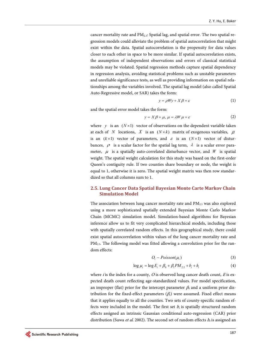
Figure 1 shows maps of PM2.5 and age adjusted lung cancer mortality rate. The
PM2.5 exhibits more clustered pattern with higher values in the east. The average
PM2.5 for all counties in the conterminous USA is 8.43 μg/m3. The eastern part
has an average value around the EPA standard limit of 12 μg/m3.The mortality
map shows some chessboard pattern but overall the east part of USA has higher
mortality rate than west, same as PM2.5. Visual comparison of the two maps re-
veals an overall positive association between PM2.5 and lung cancer mortality
rate.
3.2. ESDA
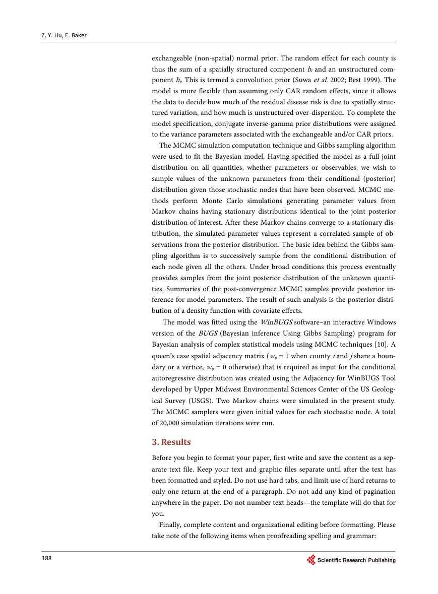
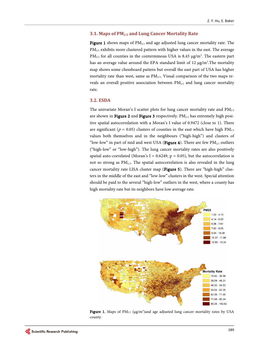
The univariate Moran’s I scatter plots for lung cancer mortality rate and PM2.5
are shown in Figure 2 and Figure 3 respectively. PM2.5 has extremely high posi-
tive spatial autocorrelation with a Moran’s I value of 0.9472 (close to 1). There
are significant (p = 0.05) clusters of counties in the east which have high PM2.5
values both themselves and in the neighbours (“high-high”) and clusters of
“low-low” in part of mid and west USA (Figure 4). There are few PM2.5 outliers
(“high-low” or “low-high”). The lung cancer mortality rates are also positively
spatial auto-correlated (Moran’s I = 0.6249, p = 0.05), but the autocorrelation is
not so strong as PM2.5. The spatial autocorrelation is also revealed in the lung
cancer mortality rate LISA cluster map (Figure 5). There are “high-high” clus-
ters in the middle of the east and “low-low” clusters in the west. Special attention
should be paid to the several “high-low” outliers in the west, where a county has
high mortality rate but its neighbors have low average rate.
Figure 1. Maps of PM2.5 (μg/m3)and age adjusted lung cancer mortality rates by USA
county.
189
�
Z. Y. Hu, E. Baker
Figure 2. PM2.5 Moran’s I scatter plot.
Figure 3. Age adjusted lung cancer mortality rate (AGEADJRATE) Moran’s I scatter plot.
The bivariate LISA cluster map is shown in Figure 6 (permutations = 500, p =
0.05). Note that this shows local patterns of spatial correlation at a county be-
tween lung cancer mortality rate and the average PM2.5 for its neighbors. Coun-
ties with significant spatial correlation are color-coded by type of spatial auto-
correlation. There are clusters of ‘high-high” (high PM2.5 in a county and high
190
�


 2023年江西萍乡中考道德与法治真题及答案.doc
 2012年重庆南川中考生物真题及答案.doc
 2013年江西师范大学地理学综合及文艺理论基础考研真题.doc
 2020年四川甘孜小升初语文真题及答案I卷.doc
 2020年注册岩土工程师专业基础考试真题及答案.doc
 2023-2024学年福建省厦门市九年级上学期数学月考试题及答案.doc
 2021-2022学年辽宁省沈阳市大东区九年级上学期语文期末试题及答案.doc
 2022-2023学年北京东城区初三第一学期物理期末试卷及答案.doc
 2018上半年江西教师资格初中地理学科知识与教学能力真题及答案.doc
 2012年河北国家公务员申论考试真题及答案-省级.doc
 2020-2021学年江苏省扬州市江都区邵樊片九年级上学期数学第一次质量检测试题及答案.doc
 2022下半年黑龙江教师资格证中学综合素质真题及答案.doc