2019ICCV_EGNet 论文原文显著性检测SOD.pdf

发布时间：2022-05-31 发布人：admin 分类：说明书资料大小：2.31M 资料格式：pdf 举报版权申诉

zjc910997316-11825874-4744302543307514023.pdf-第1页.png

第1页 / 共10页

zjc910997316-11825874-4744302543307514023.pdf-第2页.png

第2页 / 共10页

zjc910997316-11825874-4744302543307514023.pdf-第3页.png

第3页 / 共10页

zjc910997316-11825874-4744302543307514023.pdf-第4页.png

第4页 / 共10页

zjc910997316-11825874-4744302543307514023.pdf-第5页.png

第5页 / 共10页

zjc910997316-11825874-4744302543307514023.pdf-第6页.png

第6页 / 共10页

zjc910997316-11825874-4744302543307514023.pdf-第7页.png

第7页 / 共10页

zjc910997316-11825874-4744302543307514023.pdf-第8页.png

第8页 / 共10页

文本预览

IEEE International Conference on Computer Vision (ICCV) 2019 EGNet: Edge Guidance Network for Salient Object Detection Jia-Xing Zhao, Jiang-Jiang Liu, Deng-Ping Fan, Yang Cao, Ju-Feng Yang, Ming-Ming Cheng* TKLNDST, CS, Nankai University http://mmcheng.net/egnet/ Abstract Fully convolutional neural networks (FCNs) have shown their advantages in the salient object detection task. How- ever, most existing FCNs-based methods still suffer from coarse object boundaries. In this paper, to solve this prob- lem, we focus on the complementarity between salient edge information and salient object information. Accordingly, we present an edge guidance network (EGNet) for salient object detection with three steps to simultaneously model these two kinds of complementary information in a single network. In the ﬁrst step, we extract the salient object features by a progressive fusion way. In the second step, we integrate the local edge information and global loca- tion information to obtain the salient edge features. Fi- nally, to sufﬁciently leverage these complementary features, we couple the same salient edge features with salient ob- ject features at various resolutions. Beneﬁting from the rich edge information and location information in salient edge features, the fused features can help locate salient objects, especially their boundaries more accurately. Ex- perimental results demonstrate that the proposed method performs favorably against the state-of-the-art methods on six widely used datasets without any pre-processing and post-processing. The source code is available at http: //mmcheng.net/egnet/. 1. Introduction The goal of salient object detection (SOD) is to ﬁnd the most visually distinctive objects in an image. It has received widespread attention recently and been widely used in many vision and image processing related areas, such as content- aware image editing [6], object recognition [42], photo- synth [4], non-photo-realist rendering [41], weakly super- vised semantic segmentation [19] and image retrieval [15]. Besides, there are many works focusing on video salient object detection [12, 54] and RGB-D salient object detec- tion [11, 66]. Inspired by cognitive studies of visual attention [7, 21, *M.M. Cheng (cmm@nankai.edu.cn) is the corresponding author. 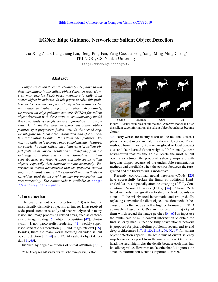Source Baseline Ours GT Figure 1. Visual examples of our method. After we model and fuse the salient edge information, the salient object boundaries become clearer. 39], early works are mainly based on the fact that contrast plays the most important role in saliency detection. These methods beneﬁt mostly from either global or local contrast cues and their learned fusion weights. Unfortunately, these hand-crafted features though can locate the most salient objects sometimes, the produced saliency maps are with irregular shapes because of the undesirable segmentation methods and unreliable when the contrast between the fore- ground and the background is inadequate. Recently, convolutional neural networks (CNNs) [25] have successfully broken the limits of traditional hand- crafted features, especially after the emerging of Fully Con- volutional Neural Networks (FCNs) [34]. These CNN- based methods have greatly refreshed the leaderboards on almost all the widely used benchmarks and are gradually replacing conventional salient object detection methods be- cause of the efﬁciency as well as high performance. In SOD approaches based on CNNs architecture, the majority of them which regard the image patches [64, 65] as input use the multi-scale or multi-context information to obtain the ﬁnal saliency map. Since the fully convolutional network is proposed for pixel labeling problems, several end-to-end deep architectures [17, 18, 23, 28, 31, 50, 60, 67] for salient object detection appear. The basic unit of output saliency map becomes per pixel from the image region. On the one hand, the result highlights the details because each pixel has its saliency value. However, on the other hand, it ignores the structure information which is important for SOD.

With the increase of the network receptive ﬁeld, the po- sitioning of salient objects becomes more and more accu- rate. However, at the same time, spatial coherence is also ignored. Recently, to obtain the ﬁne edge details, some SOD U-Net [40] based works [32, 33, 59, 61] used a bi- directional or recursive way to reﬁne the high-level features with the local information. However, the boundaries of salient objects are still not explicitly modeled. The comple- mentarity between the salient edge information and salient object information has not been noticed. Besides, there are some methods using pre-processing (Superpixel) [20] or post-processing (CRF) [17, 28, 33] to preserve the object boundaries. The main inconvenience with these approaches is their low inference speed. In this paper, we focus on the complementarity between salient edge information and salient object information. We aim to leverage the salient edge features to help the salient object features locate objects, especially their boundaries more accurately. In summary, this paper makes three major contributions: • We propose an EGNet to explicitly model complemen- tary salient object information and salient edge infor- mation within the network to preserve the salient ob- ject boundaries. At the same time, the salient edge fea- tures are also helpful for localization. • Our model jointly optimizes these two complementary tasks by allowing them to mutually help each other, which signiﬁcantly improves the predicted saliency maps. • We compare the proposed methods with 15 state-of- the-art approaches on six widely used datasets. With- out bells and whistles, our method achieves the best performance under three evaluation metrics. 2. Related Works Over the past years, some methods were proposed to de- tect the salient objects in an image. Early methods pre- dicted the saliency map using a bottom-up pattern by the hand-craft feature, such as contrast [5], boundary back- ground [57, 68], center prior [24, 44] and so on [22, 44, 51]. More details are introduced in [1, 2, 9]. Recently, Convolutional neural networks (CNNs) per- form their advantages and refresh the state-of-the-art records in many ﬁelds of computer vision. Li et al. [27] resized the image regions to three differ- ent scales to extract the multi-scale features and then aggre- gated these multiple saliency maps to obtain the ﬁnal pre- diction map. Wang et al. [45] designed a neural network to extract the local estimation for the input patches and inte- grated these features with the global contrast and geometric information to describe the image patches. However, the result is limited by the performance of image patches in these methods. In [34], long et al. ﬁrstly proposed a net- work (FCN) to predict the semantic label for each pixel. Inspired by FCN, more and more pixel-wise saliency detec- tion methods were proposed. Wang et al. [47] proposed a recurrent FCN architecture for salient object detection. Hou et al. proposed a short connection [17, 18] based on HED [55] to integrate the low-level features and high-level features to solve the scale-space problem. In [62], Zhang et al. introduced a reformulated dropout and an effective hy- brid upsampling to learn deep uncertain convolutional fea- tures to encourage robustness and accuracy. In [61], Zhang et al. explicitly aggregated the multi-level features into mul- tiple resolutions and then combined these feature maps by a bidirectional aggregation method. Zhang et al. [59] pro- posed a bi-directional message-passing model to integrate multi-level features for salient object detection. Wang et al. [53] leveraged the ﬁxation maps to help the model to locate the salient object more accurately. In [35], Luo et al. proposed a U-Net based architecture which contains an IOU edge loss to leverage the edge cues to detect the salient objects. In other saliency-related tasks, some methods of using edge cues have appeared. In [26], li et al. generated the contour of the object to obtain the salient instance seg- mentation results. In [29], li et al. leveraged the well-trained contour detection models to generate the saliency masks to overcome the limitation caused by manual annotations. Compared with most of the SOD U-Net based methods [32,33,59,61], we explicitly model edge information within the network to leverage the edge cues. Compared with the methods which use the edge cues [14,58,69], the major dif- ferences are that we use a single base network and jointly optimize the salient edge detection and the salient object de- tection, allowing them to help each other mutually. which results in better performance. Compared with NLDF [35], they implemented a loss function inspired by the Mumford- Shah function [38] to penalize errors on the edges. Since the salient edges are derived from salient objects through a ﬁxed sober operator, this penalty essentially only affects the gradient in the neighborhood of salient edges on feature maps. In this way, the edge details are optimized to some extent, but the complementarity between salient edge detec- tion and salient object detection is not sufﬁciently utilized. In our method, we design two modules to extract these two kinds of features independently. Then we fuse these com- plementary features by a one-to-one guidance module. In this way, the salient edge information can not only improve the quality of edges but also make the localization more ac- curate. The experimental part veriﬁes our statement. 3. 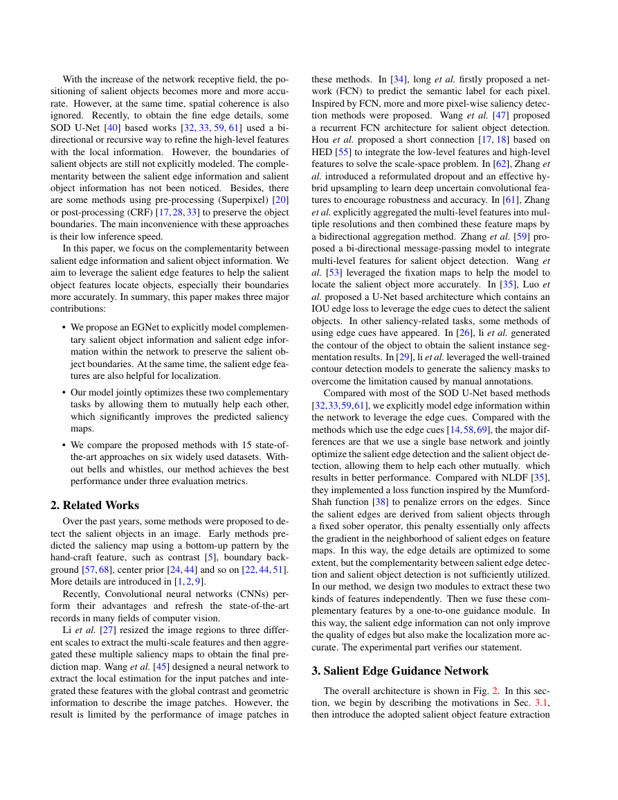Salient Edge Guidance Network The overall architecture is shown in Fig. 2. In this sec- tion, we begin by describing the motivations in Sec. 3.1, then introduce the adopted salient object feature extraction

Figure 2. The pipeline of the proposed approach. We use brown thick lines to represent information ﬂows between the scales. PSFEM: progressive salient object features extraction module. NLSEM: non-local salient edge features extraction module. O2OGM : one-to-one guidance module. FF: feature fusion. Spv.: supervision. module and the proposed non-local salient edge features ex- traction module in Sec. 3.2, and ﬁnally introduce the pro- posed one-to-one guidance module in Sec. 3.3. 3.1. Motivation The pixel-wise salient object detection methods have shown their advantages compared with region-based meth- ods. However, they ignored the spatial coherence in the images, resulting in the unsatisﬁed salient object bound- aries. Most methods [17,18,31,33,59,61] hope to solve this problem by fusing multi-scale information. Some meth- ods [17, 28, 33] used the post-processing such as CRF to reﬁne the salient object boundaries. In NLDF [35], they proposed an IOU loss to affect the gradient of the location around the edge. None of them pay attention to the com- plementarity between salient edge detection and salient ob- ject detection. A good salient edge detection result can help salient object detection task in both segmentation and local- ization, and vice versa. Based on this idea, we proposed an EGNet to model and fuse the complementary salient edge information and salient object information within a single network in an end-to-end manner. 3.2. Complementary information modeling Our proposed network is independent of the backbone network. Here we use the VGG network suggested by other deep learning based methods [17, 35] to describe the pro- posed method. First, we truncate the last three fully con- nected layers. Following DSS [17, 18], we connect another side path to the last pooling layer in VGG. Thus from the backbone network, we obtain six side features Conv1-2, Conv2-2, Conv3-3, Conv4-3, Conv5-3, Conv6-3. Because the Conv1-2 is too close to the input and the receptive ﬁeld is too small, we throw away this side path S(1). There are ﬁve side paths S(2), S(3), S(4), S(5), S(6) remaining in our method. For simplicity, these ﬁve features could be denoted by a backbone features set C: C = {C (2), C (3), C (4), C (5), C (6)}, (1) where C (2) denotes the Conv2-2 features and so on. Conv2- 2 preserves better edge information [61]. Thus we leverage the S(2) to extract the edge features and other side paths to extract the salient object features. 3.2.1 Progressive salient object features extraction As shown in PSFEM of Fig. 2, to obtain richer con- text features, we leverage the widely used architecture U- Net [40] to generate the multi-resolution features. Differ- ent from the original U-Net, in order to obtain more robust salient object features, We add three convolutional layers (Conv in Fig. 2) on each side path, and after each convo- lutional layer, a ReLU layer is added to ensure the nonlin- earity. To illustrate simply, we use the T (Tab. 1) to denote these convolutional layers and ReLU layers. Besides, deep supervision is used on each side path. We adopt a convolu- tional layer to convert the feature maps to the single-channel prediction mask and use D (Tab. 1) to denote it. The details of the convolutional layers could be found in Tab. 1. 3.2.2 Non-local salient edge features extraction In this module, we aim to model the salient edge in- formation and extract the salient edge features. As men- tioned above, the Conv2-2 preserves better edge informa- tion. Hence we extract local edge information from Conv2- 2. However, in order to get salient edge features, only local information is not enough. High-level semantic information or location information is also needed. When information U+Conv2-2Conv3-3Conv4-3Conv5-3Conv6-3ConvConvPSFEMExplicit edge modellingFFFFFFFF: Conv layerU: Upsample+: Pixel-wise addConv1-2Top-down location propagationConvConvConvNLSEMO2OGM: Saliency Spv.: Edge Spv.ConvConvConvConvConvFF

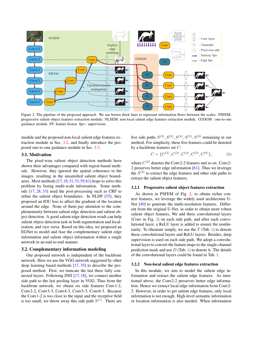
S 2 3 4 5 6 T1 1 1 2 2 3 128 256 512 512 512 3 3 5 5 7 T2 1 1 2 2 3 128 256 512 512 512 3 3 5 5 7 T3 1 1 2 2 3 128 256 512 512 512 D 1 1 1 1 1 3 3 3 3 3 1 1 1 1 1 3 3 5 5 7 Table 1. Details of each side output. T denotes the feature enhance module (Conv shown in Fig. 2). Each T contains three convolu- tional layers: T1, T2, T3 and three followed ReLu layers. We show the kernel size, padding and channel number of each convolutional layer. For example, 3, 1, 128 denote a convolutional layer whose kernel size is 3, padding is 1, channel number is 128. D denotes the transition layer which converts the multi-channel feature map to one-channel activation map. S denotes the side path. is progressively returned from the top level to the low level like the U-Net architecture, the high-level location informa- tion is gradually diluted. Besides, the receptive ﬁeld of the top-level is the largest, and the location is the most accurate. Thus we design a top-down location propagation to propa- gate the top-level location information to the side path S(2) to restrain the non-salient edge. The fused features ¯C (2) could be denoted as: ¯C (2) = C (2) + Up(φ(Trans( ˆF (6); θ)); C (2)), (2) where Trans(∗; θ) is a convolutional layer with param- eter θ, which aims to change the number of chan- nels of the feature, and φ() denotes a ReLU activa- tion function. U p(∗; C (2)) is bilinear interpolation op- eration which aims to up-sample * to the same size as C (2). On the right of the equation, the second term denotes the features from the higher side path. To il- lustrate clearly, we use UpT ( ˆF (i); θ, C (j )) to represent Up(φ(Trans( ˆF (i); θ)); C (j)). ˆF (6) denotes the enhanced features in side path S(6). The enhanced features ˆF (6) could be represented as f (C (6); W (6) T ), and the enhanced features in S(3), S(4), S(5) could be computed as: T ), ˆF (i) = f (C (i) + UpT ( ˆF (i+1); θ, C (i)); W (i) (3) T denotes the parameters in T (i) and f (∗; W (i) where W (i) T ) denotes a series of convolutional and non-linear operations with parameters W (i) T . After obtaining the guided features ¯C (2), similar with other side paths, we add a series convolutional layers to en- hance the guided feature, then the ﬁnal salient edge features FE in S(2) could be computed as f ( ¯C (2); W (2) T ). The con- ﬁguration details could be found in Tab. 1. To model the salient edge feature explicitly, we add an extra salient edge supervision to supervise the salient edge features. We use the cross-entropy loss which could be deﬁned as: L(2)(FE; W (2) log P r(yj = 1|FE; W (2) D ) D ) = − − j∈Z+ j∈Z− log P r(yj = 0|FE; W (2) D ), (4) where Z+ and Z− denote the salient edge pixels set and background pixels set, respectively. WD denotes the pa- rameters of the transition layer as shown in Tab. 1. P r(yj = 1|FE; W (2) D ) is the prediction map in which each value de- notes the salient edge conﬁdence for the pixel. In addition, the supervision added on the salient object detection side path can be represented as: D ) = − j∈Y+ L(i)( ˆF (i); W (i) − j∈Y− log P r(yj = 1| ˆF (i); W (i) D ) log P r(yj = 0| ˆF (i); W (i) D ), i ∈ [3, 6], (5) 6 where Y+ and Y− denote the salient region pixels set and non-salient pixels set, respectively. Thus the total loss L in the complementary information modeling could be denoted as: L = L(2)(FE; W (2) D ) + L(i)( ˆF (i); W (i) D ). (6) i=3 3.3. One-to-one guidance module After obtaining the complementary salient edge features and salient object features, we aim to leverage the salient edge features to guide the salient object features to perform better on both segmentation and localization. The simple way is to fuse the FE and the ˆF (3). It will be better to sufﬁ- ciently leverage the multi-resolution salient object features. However, the disadvantage of fusing the salient edge fea- tures and multi-resolution salient object features progres- sively from down to top is that salient edge features are di- luted when salient object features are fused. Besides, the goal is to fuse salient object features and salient edge fea- tures to utilize complementary information to obtain better prediction results. Hence, we propose a one-to-one guid- ance module. Moreover, experimental parts validate our view. Speciﬁcally, we add sub-side paths for S(3), S(4), S(5), S(6). In each sub-side path, by fusing the salient edge fea- tures into enhanced salient object features, we make the lo- cation of high-level predictions more accurate, and more importantly, the segmentation details become better. The salient edge guidance features (s-features) could be denoted as: G(i) = UpT ( ˆF (i); θ, FE) + FE, i ∈ [3, 6]. (7) Then similar to the PSFEM, we adopt a series of convo- lutional layers T in each sub-side path to further enhance the s-features and a transition layer D to convert the multi- channel feature map to one-channel prediction map. Here in order to illustrate clearly, we denote the T and D as T and D in this module. By Eq. (3), we obtain the enhanced s-features ˆG(i).

Here we also add deep supervision for these enhanced s- features. For each sub-side output prediction map, the loss can be calculated as: L(i) D ) = − log P r(yj = 1| ˆG(i); W (i) D ) ( ˆG(i); W (i) j∈Y+ log P r(yj = 0| ˆG(i); W (i) D ), i ∈ [3, 6]. (8) − j∈Y− Then we fuse the multi-scale reﬁned prediction maps to ob- tain a fused map. The loss function for the fused map can be denoted as: L f ( ˆG; WD) = σ(Y, βif ( ˆG(i); W (i) D )), (9) where the σ(∗,∗) represents the cross-entropy loss between prediction map and saliency ground-truth, which has the same form to Eq. (5). Thus the loss for this part and the total for the proposed network could be expressed as: 6 i=3 i=6 i=3 f ( ˆG; WD) + L = L Lt = L + L. L(i) ( ˆG(i); W (i) D ) (10) 4. Experiments 4.1. Implementation Details We train our model on DUTS [46] dataset followed by [33,49,59,63]. For a fair comparison, we use VGG [43] and ResNet [16] as backbone networks, respectively. Our model is implemented in PyTorch. All the weights of newly added convolution layers are initialized randomly with a truncated normal (σ = 0.01), and the biases are initialized to 0. The hyper-parameters are set as followed: learning rate = 5e- 5, weight decay = 0.0005, momentum = 0.9, loss weight for each side output is equal to 1. A back propagation is processing for each of the ten images. We do not use the validation dataset during training. We train our model 24 epochs and divide the learning rate by 10 after 15 epochs. During inference, we are able to obtain a predicted salient edge map and a set of saliency maps. In our method, we directly use the fused prediction map as the ﬁnal saliency map. 4.2. Datasets and Evaluation Metric We have evaluated the proposed architecture on six widely used public benchmark datasets: ECSSD [56], PASCAL-S [30], DUT-OMRON [57], SOD [36, 44], HKU- IS [27], DUTS [46]. ECSSD [56] contains 1000 meaningful semantic images with various complex scenes. PASCAL- S [30] contains 850 images which are chosen from the vali- dation set of the PASCAL VOC segmentation dataset [8]. DUT-OMRON [57] contains 5168 high-quality but chal- lenging images. Images in this dataset contain one or more salient objects with a relatively complex background. SOD [36] contains 300 images and is proposed for image seg- mentation. Pixel-wise annotations of salient objects are generated by [44]. It is one of the most challenging datasets currently. HKU-IS [27] contains 4447 images with high- quality annotations, many of which have multiple discon- nected salient objects. This dataset is split into 2500 train- ing images, 500 validation images and 2000 test images. DUTS [46] is the largest salient object detection bench- mark. It contains 10553 images for training and 5019 im- ages for testing. Most images are challenging with var- ious locations and scales. Following most recent works [33, 49, 52], we use the DUTS dataset to train the proposed model. We use three widely used and standard metrics, F- measure, mean absolute error (MAE) [2], and a recently proposed structure-based metric, namely S-measure [10], to evaluate our model and other state-of-the-art models. F- measure is a harmonic mean of average precision and aver- age recall, formulated as: Fβ = (1 + β2)P recision × Recall β2 × P recision + Recall , (11) we set β2 = 0.3 to weigh precision more than recall as suggested in [5]. Precision denotes the ratio of detected salient pixels in the predicted saliency map. Recall denotes the ratio of detected salient pixels in the ground-truth map. Precision and recall are computed on binary images. Thus we should threshold the prediction map to binary map ﬁrst. There are different precision and recall of different thresh- olds. We could plot the precision-recall curve at different thresholds. Here we use the code provided by [17, 18] for evaluation. Following most salient object detection meth- ods [17,18,32,59], we report the maximum F-measure from all precision-recall pairs. MAE is a metric which evaluates the average difference between prediction map and ground-truth map. Let P and Y denote the saliency map and the ground truth that is nor- malized to [0, 1]. We compute the MAE score by: ε = 1 W × H |P (x, y) − Y (x, y)|, (12) W H x=1 y=1 where W and H are the width and height of images, respec- tively. S-measure focuses on evaluating the structural informa- tion of saliency maps, which is closer to the human visual system than F-measure. Thus we include S-measure for a more comprehensive evaluation. S-measure could be com- puted as: S = γSo + (1 − γ)Sr, (13)

ECSSD [56] PASCAL-S [30] DUT-O [57] HKU-IS [27] SOD [36, 37] DUTS-TE [46] MaxF ↑ MAE ↓ S ↑ MaxF ↑ MAE ↓ S ↑ MaxF ↑ MAE ↓ S ↑ MaxF ↑ MAE ↓ S ↑ MaxF ↑ MAE ↓ S ↑ MaxF ↑ MAE ↓ S ↑ DCL∗ [28] DSS∗ [17, 18] MSR [26] NLDF [35] RAS [3] ELD∗ [13] DHS [32] RFCN∗ [48] UCF [62] Amulet [61] C2S [29] PAGR [63] Ours 0.896 0.906 0.903 0.903 0.915 0.865 0.905 0.898 0.908 0.911 0.909 0.924 0.941 0.080 0.064 0.059 0.065 0.060 0.082 0.062 0.097 0.080 0.062 0.057 0.064 0.044 0.863 0.882 0.875 0.875 0.886 0.839 0.884 0852 0.884 0.894 0.891 0.889 0.913 0.805 0.821 0.839 0.822 0.830 0.772 0.825 0.827 0.820 0.826 0.845 0.847 0.863 0.115 0.101 0.083 0.098 0.102 0.122 0.092 0.118 0.127 0.092 0.081 0.089 0.076 0.791 0.796 0.802 0.803 0.798 0.757 0.807 0.799 0.806 0.820 0.839 0.818 0.848 0.733 0.760 0.790 0.753 0.784 0.738 - 0.747 0.735 0.737 0.759 0.771 0.826 0.893 0.900 0.907 0.902 0.910 0.843 0.892 0.895 0.888 0.889 0.897 0.919 0.929 0.063 0.050 0.043 0.048 0.047 0.072 0.052 0.079 0.073 0.052 0.047 0.047 0.034 0.859 0.878 0.852 0.878 0.884 0.823 0.869 0.860 0.874 0.886 0.886 0.889 0.910 0.831 0.834 0.841 0.837 0.844 0.762 0.823 0.805 0.798 0.799 0.821 0.841 0.869 0.131 0.125 0.111 0.123 0.130 0.154 0.128 0.161 0.164 0.146 0.122 0.146 0.110 0.748 0.744 0.757 0.756 0.760 0.705 0.750 0.730 0.762 0.753 0.763 0.716 0.788 0.786 0.813 0.824 0.816 0.800 0.747 0.815 0.786 0.771 0.773 0.811 0.854 0.880 0.081 0.065 0.062 0.065 0.060 0.092 0.065 0.090 0.116 0.075 0.062 0.055 0.043 0.785 0.812 0.809 0.805 0.827 0.749 0.809 0.784 0.777 0.796 0.822 0.825 0.866 VGG-based 0.094 0.074 0.073 0.079 0.063 0.093 0.743 0.765 0.767 0.750 0.792 0.743 - - 0.752 0.094 0.748 0.131 0.771 0.083 0.783 0.072 0.751 0.071 0.056 0.813 ResNet-based 0.777 0.069 0.062 0.791 0.808 0.064 0.052 0.818 0.769 0.774 0.820 0.842 0.838 0.844 0.864 0.869 0.916 0.921 0.932 0.943 0.056 0.043 0.048 0.041 0.895 0.906 0.914 0.918 SRM∗ [49] 0.824 DGRL [52] 0.836 PiCANet∗ [33] 0.850 Ours 0.875 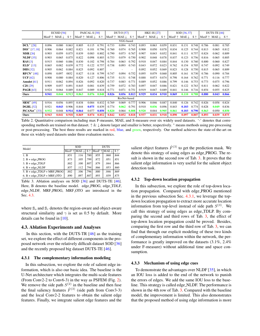Table 2. Quantitative comparison including max F-measure, MAE, and S-measure over six widely used datasets. ‘-’ denotes that corre- sponding methods are trained on that dataset. ↑ & ↓ denote larger and smaller is better, respectively. ∗ means methods using pre-processing or post-processing. The best three results are marked in red, blue, and green, respectively. Our method achieves the state-of-the-art on these six widely used datasets under three evaluation metrics. 0.046 0.036 0.044 0.031 0.126 0.103 0.103 0.097 0.058 0.049 0.050 0.039 0.084 0.075 0.077 0.074 0.887 0.896 0.905 0.918 0.742 0.774 0.790 0.807 0.832 0.839 0.850 0.852 0.906 0.910 0.920 0.937 0.840 0.843 0.861 0.890 0.826 0.828 0.863 0.893 SOD DUTS Model MaxF ↑ MAE ↓ S ↑ MaxF ↑ MAE ↓ S ↑ .844 .851 1. B .851 .873 2. B + edge PROG .882 .866 3. B + edge TDLP .860 4. B + edge NLDF .857 .869 5. B + edge TDLP + MRF PROG .882 6. B + edge TDLP + MRF OTO .890 .875 Table 3. Ablation analyses on SOD [36] and DUTS-TE [46]. Here, B denotes the baseline model. edge PROG, edge TDLF, edge NLDF, MRF PROG, MRF OTO are introduced in the Sec. 4.3. .116 .105 .100 .112 .106 .097 .780 .799 .807 .794 .796 .807 .855 .872 .879 .866 .880 .893 .060 .051 .044 .053 .046 .039 where So and Sr denotes the region-aware and object-aware structural similarity and γ is set as 0.5 by default. More details can be found in [10]. 4.3. Ablation Experiments and Analyses In this section, with the DUTS-TR [46] as the training set, we explore the effect of different components in the pro- posed network over the relatively difﬁcult dataset SOD [36] and the recently proposed big dataset DUTS-TE [46]. 4.3.1 The complementary information modeling In this subsection, we explore the role of salient edge in- formation, which is also our basic idea. The baseline is the U-Net architecture which integrates the multi-scale features (From Conv2-2 to Conv6-3) in the way as PSFEM (Fig. 2). We remove the side path S(2) in the baseline and then fuse the ﬁnal saliency features ˆF (3) (side path from Conv3-3) and the local Conv2-2 features to obtain the salient edge features. Finally, we integrate salient edge features and the salient object features ˆF (3) to get the prediction mask. We denote this strategy of using edges as edge PROG. The re- sult is shown in the second row of Tab. 3. It proves that the salient edge information is very useful for the salient object detection task. 4.3.2 Top-down location propagation In this subsection, we explore the role of top-down loca- tion propagation. Compared with edge PROG mentioned in the previous subsection Sec. 4.3.1, we leverage the top- down location propagation to extract more accurate location information from top-level instead of side path S(3). We call this strategy of using edges as edge TDLP. By com- paring the second and third rows of Tab. 3, the effect of top-down location propagation could be proved. Besides, comparing the ﬁrst row and the third row of Tab. 3, we can ﬁnd that through our explicit modeling of these two kinds of complementary information within the network, the per- formance is greatly improved on the datasets (3.1%, 2.4% under F-measure) without additional time and space con- sumption. 4.3.3 Mechanism of using edge cues To demonstrate the advantages over NLDF [35], in which an IOU loss is added to the end of the network to punish the errors of edges. We add the same IOU loss to the base- line. This strategy is called edge NLDF. The performance is shown in the 4th row of Tab. 3. Compared with the baseline model, the improvement is limited. This also demonstrates that the proposed method of using edge information is more

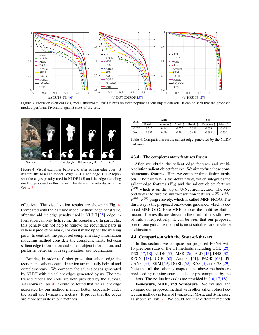
(a) DUTS-TE [46] (b) DUT-OMRON [57] (c) HKU-IS [27] Figure 3. Precision (vertical axis) recall (horizontal axis) curves on three popular salient object datasets. It can be seen that the proposed method performs favorably against state-of-the-arts. 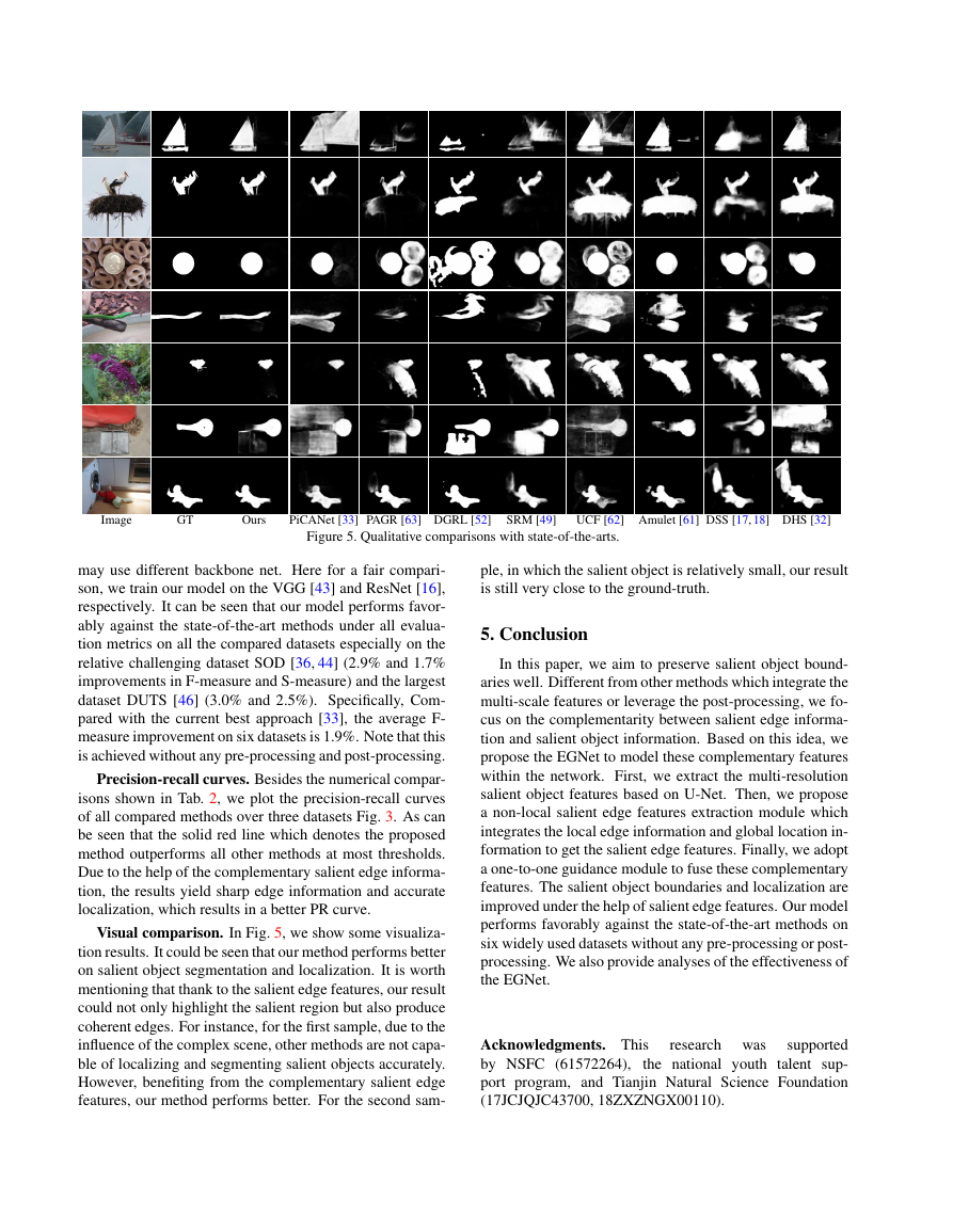Model NLDF Ours Recall ↑ 0.513 0.637 SOD Precision ↑ MaxF ↑ Recall ↑ 0.318 0.446 0.541 0.534 0.527 0.581 DUTS Precision ↑ MaxF ↑ 0.429 0.539 0.659 0.680 Source B B+edge NLDF B+edge TDLP GT Figure 4. Visual examples before and after adding edge cues. B denotes the baseline model. edge NLDF and edge TDLP repre- sent the edges penalty used in NLDF [35] and the edge modeling method proposed in this paper. The details are introduced in the Sec. 4.3. effective. The visualization results are shown in Fig. 4. Compared with the baseline model without edge constraint, after we add the edge penalty used in NLDF [35], edge in- formation can only help reﬁne the boundaries. In particular, this penalty can not help to remove the redundant parts in saliency prediction mask, nor can it make up for the missing parts. In contrast, the proposed complementary information modeling method considers the complementarity between salient edge information and salient object information, and performs better on both segmentation and localization. Besides, in order to further prove that salient edge de- tection and salient object detection are mutually helpful and complementary. We compare the salient edges generated by NLDF with the salient edges generated by us. The pre- trained model and code are both provided by the authors. As shown in Tab. 4, it could be found that the salient edge generated by our method is much better, especially under the recall and F-measure metrics. It proves that the edges are more accurate in our methods. Table 4. Comparisons on the salient edge generated by the NLDF and ours. 4.3.4 The complementary features fusion After we obtain the salient edge features and multi- resolution salient object features. We aim to fuse these com- plementary features. Here we compare three fusion meth- ods. The ﬁrst way is the default way, which integrates the salient edge features (FE) and the salient object features ˆF (3) which is on the top of U-Net architecture. The sec- ond way is to fuse the multi-resolution features ˆF (3), ˆF (4), ˆF (5), ˆF (6) progressively, which is called MRF PROG. The third way is the proposed one-to-one guidance, which is de- noted MRF OTO. Here MRF denotes the multi-resolution fusion. The results are shown in the third, ﬁfth, sixth rows of Tab. 3, respectively. It can be seen that our proposed one-to-one guidance method is most suitable for our whole architecture. 4.4. Comparison with the State-of-the-art In this section, we compare our proposed EGNet with 15 previous state-of-the-art methods, including DCL [28], DSS [17, 18], NLDF [35], MSR [26], ELD [13], DHS [32], RFCN [48], UCF [62], Amulet [61], PAGR [63], Pi- CANet [33], SRM [49], DGRL [52], RAS [3] and C2S [29]. Note that all the saliency maps of the above methods are produced by running source codes or pre-computed by the authors. The evaluation codes are provided in [10, 17, 18]. F-measure, MAE, and S-measure. We evaluate and compare our proposed method with other salient object de- tection methods in term of F-measure, MAE, and S-measure as shown in Tab. 2. 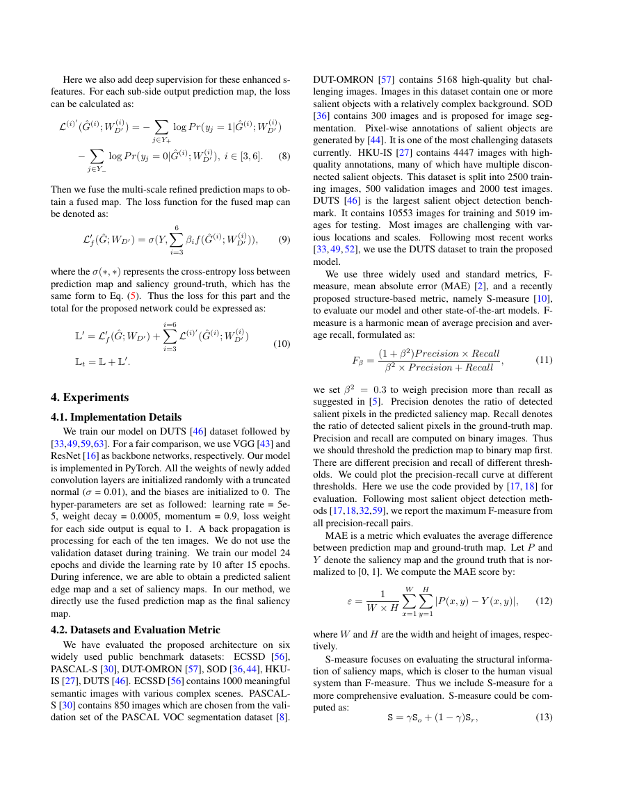We could see that different methods 00.20.40.60.810.60.70.80.91DCLRFCNMSRDSSAmuletSRMPAGRDGRLPiCANetOurs00.20.40.60.810.60.70.80.91DCLRFCNMSRDSSAmuletSRMPAGRDGRLPiCANetOurs00.20.40.60.810.60.70.80.91DCLRFCNMSRDSSAmuletSRMPAGRDGRLPiCANetOurs

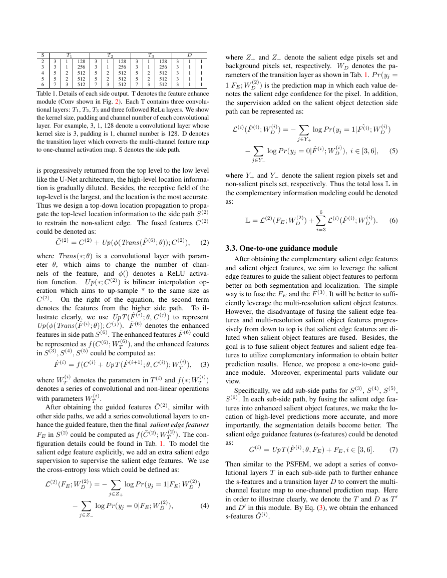
Image GT Ours PiCANet [33] PAGR [63] DGRL [52] SRM [49] UCF [62] Amulet [61] DSS [17, 18] DHS [32] Figure 5. Qualitative comparisons with state-of-the-arts. may use different backbone net. Here for a fair compari- son, we train our model on the VGG [43] and ResNet [16], respectively. It can be seen that our model performs favor- ably against the state-of-the-art methods under all evalua- tion metrics on all the compared datasets especially on the relative challenging dataset SOD [36, 44] (2.9% and 1.7% improvements in F-measure and S-measure) and the largest dataset DUTS [46] (3.0% and 2.5%). Speciﬁcally, Com- pared with the current best approach [33], the average F- measure improvement on six datasets is 1.9%. Note that this is achieved without any pre-processing and post-processing. Precision-recall curves. Besides the numerical compar- isons shown in Tab. 2, we plot the precision-recall curves of all compared methods over three datasets Fig. 3. As can be seen that the solid red line which denotes the proposed method outperforms all other methods at most thresholds. Due to the help of the complementary salient edge informa- tion, the results yield sharp edge information and accurate localization, which results in a better PR curve. Visual comparison. In Fig. 5, we show some visualiza- tion results. It could be seen that our method performs better on salient object segmentation and localization. It is worth mentioning that thank to the salient edge features, our result could not only highlight the salient region but also produce coherent edges. For instance, for the ﬁrst sample, due to the inﬂuence of the complex scene, other methods are not capa- ble of localizing and segmenting salient objects accurately. However, beneﬁting from the complementary salient edge features, our method performs better. For the second sam- ple, in which the salient object is relatively small, our result is still very close to the ground-truth. 5. Conclusion In this paper, we aim to preserve salient object bound- aries well. Different from other methods which integrate the multi-scale features or leverage the post-processing, we fo- cus on the complementarity between salient edge informa- tion and salient object information. Based on this idea, we propose the EGNet to model these complementary features within the network. First, we extract the multi-resolution salient object features based on U-Net. Then, we propose a non-local salient edge features extraction module which integrates the local edge information and global location in- formation to get the salient edge features. Finally, we adopt a one-to-one guidance module to fuse these complementary features. The salient object boundaries and localization are improved under the help of salient edge features. Our model performs favorably against the state-of-the-art methods on six widely used datasets without any pre-processing or post- processing. We also provide analyses of the effectiveness of the EGNet. Acknowledgments. This supported by NSFC (61572264), the national youth talent sup- port program, and Tianjin Natural Science Foundation (17JCJQJC43700, 18ZXZNGX00110). research was

分享到：

赞收藏

资料库

2019ICCV_EGNet 论文原文显著性检测SOD.pdf

相关推荐

人工智能

热门标签

最新资料