Applied Mathematics, 2018, 9, 512-535
http://www.scirp.org/journal/am
ISSN Online: 2152-7393
ISSN Print: 2152-7385
Nonlinear Differential Equation of
Macroeconomic Dynamics for Long-Term
Forecasting of Economic Development
Askar Akaev
Prigogine Institute of Mathematical Investigations of Complex Systems, Moscow State University, Moscow, Russia
How to cite this paper: Akaev, A. (2018)
Nonlinear Differential Equation of Ma-
croeconomic Dynamics
for Long-Term
Forecasting of Economic Development.
Applied Mathematics, 9, 512-535.
https://doi.org/10.4236/am.2018.95037
Received: March 20, 2018
Accepted: May 27, 2018
Published: May 30, 2018
Copyright © 2018 by author and
Scientific Research Publishing Inc.
This work is licensed under the Creative
Commons Attribution International
License (CC BY 4.0).
http://creativecommons.org/licenses/by/4.0/
Open Access
Abstract
In this article we derive a general differential equation that describes
long-term economic growth in terms of cyclical and trend components. Equa-
tion is based on the model of non-linear accelerator of induced investment. A
scheme is proposed for obtaining approximate solutions of nonlinear diffe-
rential equation by splitting solution into the rapidly oscillating business
cycles and slowly varying trend using Krylov-Bogoliubov-Mitropolsky aver-
aging. Simplest modes of the economic system are described. Characteristics
of the bifurcation point are found and bifurcation phenomenon is interpreted
as loss of stability making the economic system available to structural change
and accepting innovations. System being in a nonequilibrium state has a dy-
namics with self-sustained undamped oscillations. The model is verified with
economic development of the US during the fifth Kondratieff cycle
(1982-2010). Model adequately describes real process of economic growth in
both quantitative and qualitative aspects. It is one of major results that the
model gives a rough estimation of critical points of system stability loss and
falling into a crisis recession. The model is used to forecast the macroeco-
nomic dynamics of the US during the sixth Kondratieff cycle (2018-2050). For
this forecast we use fixed production capital functional dependence on a
long-term Kondratieff cycle and medium-term Juglar and Kuznets cycles.
More accurate estimations of the time of crisis and recession are based on the
model of accelerating log-periodic oscillations. The explosive growth of the
prices of highly liquid commodities such as gold and oil is taken as real pre-
dictors of the global financial crisis. The second wave of crisis is expected to
come in June 2011.
Keywords
Long-Term Economic Trend, Cycles, Nonlinear Accelerator, Induced and
DOI: 10.4236/am.2018.95037 May 30, 2018
512
Applied Mathematics
�
A. Akaev
Autonomous Investment, Differential Equations of Macroeconomic Dynamics,
Bifurcation, Stability, Crisis Recession, Forecasting, Explosive Growth in the
Prices of Highly Liquid Commodities as a Predictor of Crisis
1. Introduction
Economy usually fluctuates around its trend path. These fluctuations are cyclical,
but irregular. Trend is the result of the factors responsible for long-term growth
of the economy, such as capital inflows, manpower increase, scientific and tech-
nical progress. Business cycles represent deviations of the real aggregate output
from its long-term trend caused by distributed in time random supply shocks. In
1950s there were developed some elegant mathematical models of the theory of
cycles based on the mechanism of interaction between the multiplier and acce-
lerator [1], as well as neoclassical growth theories using the production functions
[2]. They became the starting point for all subsequent research in these two cen-
tral issues of macroeconomic dynamics. The main drawback of these models was
an isolated consideration of growth and cyclical fluctuations, whereas the
Schumpeterian theory of economic development [3] [4] states that cyclical fluc-
tuations are an integral part of sustainable economic growth. Therefore, the
theory of real business cycles (RBC) must necessarily include the interaction of
the mechanisms of growth and cyclical fluctuations. The tenets of the discrete
RBC theory were laid in the 1980s by Nobel laureates F. Kydland and E. Prescott
[5]. They developed an RBC model based on stochastic dynamic model of gen-
eral equilibrium. Their model included a stochastic version of the neoclassical
Solow’s growth model [2]. Kydland’s and Prescott’s discrete RBC model became
the basic one in macroeconomic computer simulation.
2. Derivation of the Macroeconomic Dynamics Equation
Describing the Interaction of Long-Term Growth and
Business Cycles
Our first attempt to create a continuous RBC model was described in [6]. This is
a general differential equation of macroeconomic dynamics based on the inte-
raction of the mechanisms of growth and cyclical fluctuations. Let us start de-
riving this equation following the most fruitful scheme formerly chosen by Phil-
lips [1]. In this scheme it is assumed that the planned values for consumption
and investment are achieved. We also take this starting point. Hence consump-
tion and investment plans (with a certain lag) turn into actual costs, which give a
total output. If you select the expenditures (independent from revenue) A on
capital investment and consumption, the basic equilibrium condition is written
as
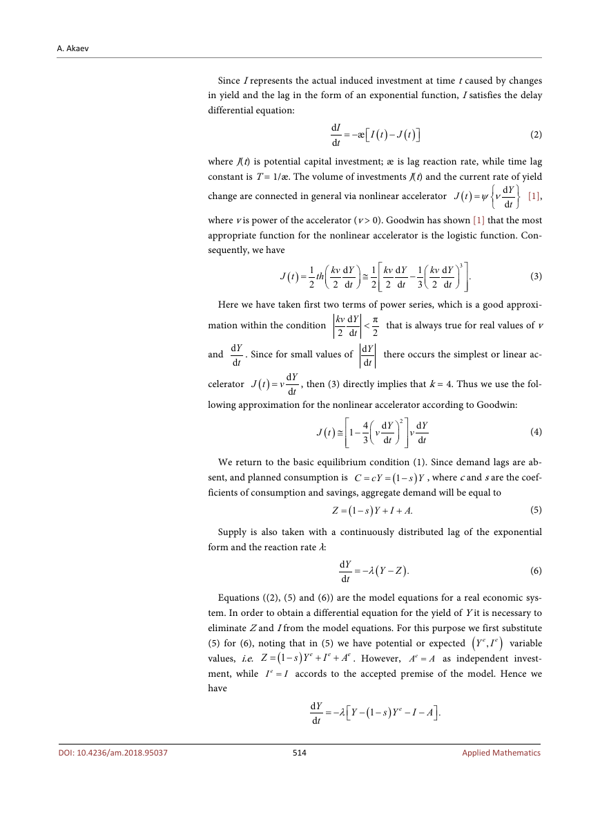
Y C I A
+ + , (1)
=
DOI: 10.4236/am.2018.95037
where C is consumption; I is actual induced investment.
513
Applied Mathematics
�
A. Akaev
Since I represents the actual induced investment at time t caused by changes
in yield and the lag in the form of an exponential function, I satisfies the delay
differential equation:
I
d
t
d
= −
æ
( )
I t
−
( )
J t
(2)
where J(t) is potential capital investment; æ is lag reaction rate, while time lag
constant is T = 1/æ. The volume of investments J(t) and the current rate of yield
[1],
change are connected in general via nonlinear accelerator
( )
J t
ψ ν
=
Y
d
t
d
where v is power of the accelerator (v > 0). Goodwin has shown [1] that the most
appropriate function for the nonlinear accelerator is the logistic function. Con-
sequently, we have
( )
J t
=
1
2
th
kv Y
d
t
2 d
≅
kv Y
d
1
t
2 2 d
−
kv Y
d
1
t
3 2 d
3
.
(3)
Here we have taken first two terms of power series, which is a good approxi-
that is always true for real values of v
<
mation within the condition
Y
and d
t
d
Y
. Since for small values of d
t
d
kv Y
d
t
2 d
π
2
there occurs the simplest or linear ac-
celerator
( )
J t
=
v
, then (3) directly implies that k = 4. Thus we use the fol-
lowing approximation for the nonlinear accelerator according to Goodwin:
Y
d
t
d
( )
J t
≅
1
−
4
3
v
Y
d
t
d
2
v
Y
d
t
d
(4)
We return to the basic equilibrium condition (1). Since demand lags are ab-
, where c and s are the coef-
sent, and planned consumption is
ficients of consumption and savings, aggregate demand will be equal to
C сY
(
1
= −
)
s Y
=
(5)
Supply is also taken with a continuously distributed lag of the exponential
)
s Y I A
.
+ +
(
1
= −
Z
form and the reaction rate λ:
Y
d
t
d
(
λ= −
Y Z
−
)
.
(6)
Equations ((2), (5) and (6)) are the model equations for a real economic sys-
tem. In order to obtain a differential equation for the yield of Y it is necessary to
eliminate Z and I from the model equations. For this purpose we first substitute
(5) for (6), noting that in (5) we have potential or expected (
variable
(
Z
1
= −
as independent invest-
values, i.e.
ment, while
I= accords to the accepted premise of the model. Hence we
eI
have
. However,
,e
Y I
)
s Y
A=
e
A
eA
+
+
)
e
I
e
e
DOI: 10.4236/am.2018.95037
Y
d
t
d
= −
λ
Y
(
1
− −
)
s Y
e
− −
I A
.
514
Applied Mathematics
�
Solving the last equation for I and differentiating the resulting expression we
obtain, respectively:
A. Akaev
I
I
d
t
d
=
=
Y
1 d
tλ
d
2
Y
1 d
2
tλ
d
+
(
1
+ − −
Y
)
s Y
e
−
A
;
Y
d
t
d
(
1
− −
)
s
e
Y
d
t
d
−
YA
d
t
d
.
Substituting these expressions into Equation (2) we obtain the following dif-
ferential equation for the yield Y:
1
2
Y
d
2
t
d
λ
æ æ
+ −
v
λ
+
−
4
χ
3
v
Y
d
t
d
+
(
Y
æ 1
æ
λ λ
−
−
)
s Y
e
=
2
A
d
λ
t
d
Y
d
t
d
−
(
1
λ
−
)
s
e
Y
d
t
d
æ Aλ+
(7)
Here constant χ takes only two values, 0 or 1. At
Phillips model with a linear accelerator, and if
model with nonlinear accelerator [1].
Y Y=
If in Equation (7) we assume
e
0χ= we have the classic
1χ= we have the Phillips-Goodwin
since yield Y is an unplanned value, and if we set
then we come to the well-known equation of Phillips [1]:
, which is a very rough approximation,
as well,
0χ= and
const
А =
2
Y
d
2
t
d
+
(
s
λ
+ −
æ æ
v
λ
)
Y
d
t
d
+
æ
λ
sY
=
A
æ .
λ
Unlike Phillips and Goodwin, we will include into (7) an expression for the
potential (expected) value of yield
eY defined by the basic factors of produc-
tion, i.e. capital (K) and labor (L). As it is well known [2], the connection of yield
with factors of production is determined by the production function of the form
, which represents the trajectory of long-term economic growth.
Y F K L
Since the production functions possess the homogeneity property, they satisfy
Euler’s equation [7]:
=
(
)
,
aK
Y
∂
K
∂
+
bL
Y
∂
L
∂
=
hY
,
where a, b and h are constant coefficients. This implies the desired approximate
expression for the expected value of
a
h
eY yield:
Y
b
∂
K h
∂
Y
∂
L
∂
(8)
K
Y
Y
L
≅
=
+
e
.
It is obvious that this approximation is more accurate than the very rough
. But the main advantage of this approach is that it
Phillips’s assumption
provides an opportunity to introduce production factors into the basic equation.
Differentiating (8) on time and performing the necessary simplification, we ob-
tain:
Y Y=
e
DOI: 10.4236/am.2018.95037
eY
d
t
d
≅
Y K
d
∂
K t
d
∂
+
Y L
d .
∂
L t
d
∂
(9)
515
Applied Mathematics
�
A. Akaev
L
It is necessary to exclude d
t
d
establishing the relationship between change in unemployment rate ( и и∗−
change in yield ( FY
from here. For this we use the Okun’s law [8]
Y− ):
) and
Y
Y
−
F
Y
F
=
(
γ
∗
u u
−
)
. (10)
(
FY L∗
)
)
2 3
γ= ÷ );
Here γ is Okun’s parameter (
is the national income at full
(
employment,
Y L is the actual yield in the presence of market unemployment;
L* is the number of workers at full employment; L is the actual number of work-
ers employed in production; u* is the natural rate of unemployment corres-
ponding to full employment L*; u is the actual level of unemployment. As
∗
L
L
, then from (10) it follows that
−
∗
L
. Differentiating both sides of this relation, we obtain the required ex-
, where
− =
FY
γ∗
∗
L
Y
L
−
(
)
и и
−
∗
=
=
γ γ∗
FY
∗
L
pression:
L
d
t
d
Y
1 d
tγ∗=
d
. (11)
As is known, the average labor productivity
KY
*
L
is associated with extreme
(marginal) labor productivity
∂
Y
∂
L
as follows [9]:
Y
∂
L
∂
≅
β
FY
*
L
. Therefore,
*
γ
=
γ
β
Y
∂
L
∂
. (12)
Substituting (11) and (12) into the initial expression (9), we obtain:
eY
d
t
d
+
=
Y
d
t
d
Y K
d
∂
K t
d
∂
β
γ
eY
eY (8) and d
t
d
. (13)
(13) into Equation (7). As a
Now it remains to substitute
result, we obtain the desired total differential equation of macroeconomic dy-
namics:
d
d
2
Y
2
t
+
+ −
æ æ
(
1
λ λ
−
v
λ
−
)
s
β
γ
+
χ λ
æ
4
3
v v
Y
d
t
d
2
Y
d
t
d
+
(
Y
æ 1
æ
λ λ
−
−
)
s Y
−
(
1
λ
−
)
s
Y K
d
∂
K t
d
∂
=
λ
A
d
t
d
+
æ
A
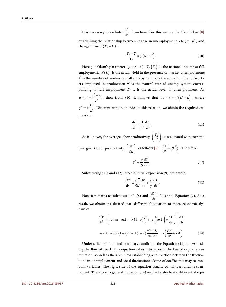
(14)
Under suitable initial and boundary conditions the Equation (14) allows find-
ing the flow of yield. This equation takes into account the law of capital accu-
mulation, as well as the Okun law establishing a connection between the fluctua-
tions in unemployment and yield fluctuations. Some of coefficients may be ran-
dom variables. The right side of the equation usually contains a random com-
ponent. Therefore in general Equation (14) we find a stochastic differential equ-
516
Applied Mathematics
DOI: 10.4236/am.2018.95037
�
A. Akaev
( )Y t
= − , and slowly varying
. This approach makes it relatively easy to find both dependences.
ation, combining deterministic and stochastic approaches of the study of real busi-
ness cycles. In this equation, we are dealing with two variables that characterize the
yield: the rapidly changing variable Y(t), which contains the cyclical fluctuations
, representing the trend curve. This circums-
y Y Y
tance makes it possible to separate them using Krylov-Bogoliubov-Mitropolsky av-
eraging [10]. Indeed, we can first average the rapidly changing variable y(t) and
get a simplified description of the system dynamics—long-term trend described
by
( )Y t
For further analysis of Equation (14) it is important to distinguish the trend
component in its right side, which is determined by the investments indepen-
dent from income. This includes the investment of public and private organiza-
tions into the development of public infrastructure, and investment caused by
scientific and technological progress, inventions and technological innovations
that not only define the long-term growth, but also affect the short-term fluctua-
tions, since they are irregular. It also includes independent expenditures on
household consumption. Thus, the independent investment
can always
be represented as
is trend component (e.g.,
( )
( )tϕ is quasi-periodic function oscillating around the trend
A t
component. Thus, the right side of the equation becomes:
æ
ϕ
. (15)
d
ϕ
+
t
d
, where
( )
tϕ
( )
A t
( )
А t
( )A t
A
d
t
d
A
d
t
d
( )A t
0egt
A=
);
æ
æ
A
A
=
+
+
=
+
+
The second term on the right side of this expression has a direct influence on
cyclical fluctuations.
First of all, we distinguish in the basic Equation (14) the cyclical fluctuations
2
described by the variable y Y Y
= − . For this, first, the nonlinear term
ν
Y
d
t
d
will replace with approximation
2
ν
y
d
t
d
to use the principle of superposition,
because Y is a slowly varying function in comparison with Y or y. Moreover,
)0
.
this nonlinear term is retained only with
Substituting Y
2
d
t
d
= + into the Equation (14) we obtain:
y Y
y
y
d
s
−
+
2
t
d
(
1
σ ω λ
and lacks with
Y K
d
∂
K t
d
∂
2
σ ω
(
y χ=
Y χ=
)1
2
Y
+
+
+
+
−
y
(
)
(16)
2
Y
d
2
t
d
d
ϕ
+
t
d
Y
d
t
d
æ .
ϕ
=
λ
A
d
t
d
+
æ
A
+
λ
Here
2
æ;
ω λ=
(17)
σ λ
æ 1 s
= + − −
(
)
λ
β
γ
−
v
æ
λ
1
−
2
4
3
v
y
d
t
d
2
ω λ=
æ ;s
σ λ
= + −
æ æ
v
λ
(
1
− −
s
;
)
λ
β
.
γ
DOI: 10.4236/am.2018.95037
As Y
∂
L
∂
and Y
∂
K
∂
are both slowly varying functions they can be replaced by
517
Applied Mathematics
�
A. Akaev
the expressions obtained from profit maximization within the model of perfect
competition [7]:
Y
∂
K
∂
=
i
;
Y
∂
L
∂
=
w
≅
,FY
β ∗
L
where the i is rate of interest; w is real wages; β reflects the elasticity of output to
labor in the Cobb-Douglas production function. We have already used earlier
the second of these relations. Therefore Equation (16) has the form:
d
d
2
t
y
2
+
2
δ ω
+
y
d
t
d
y
+
=
λ
A
d
t
d
+
æ
A
+
λ
2
Y
d
2
t
d
d
ϕ
+
t
d
Y
d
t
d
(
æ
1
ϕ λ
+
+
δ
+
2
Y
ω
(18)
−
)
s i
K
d
t
d
.
At the next step we use averaging on (18) for rapidly changing variables y and
φ and get a simplified differential equation that describes only its trend trajecto-
ry:
d
d
2
Y
2
t
+
σ ω λ
Y
d
t
d
2
Y
+
=
A
d
t
d
+
æA
+
(
1
λ
−
)
s i
K
d
t
d
=
( )
F t
1
. (19)
Initial conditions are as follows:
Y
t T
=
0
=
Y
0
Y
d;
t
d
t T
=
0
=
x
0
.
(20)
t
2
y
=
+
+
y
d
t
d
æ
ϕ
d
ϕ
+
t
d
σ ω λ
describing the cyclical fluctuations. In this
The principle of averaging leads to the equation
2
y
2
d
d
equation we must take into account the nonlinearity of the accelerator com-
prised in the coefficient σ (17). Therefore, we will analyze the solution of the
nonlinear differential equation in the form:
2
( )
y F t
σ
0
(21)
y
d
t
d
y
d
t
d
v
æ
λ
d
d
2
ω
4
3
y
2
2
t
−
−
=
2
+
,
3
where
σ
0
= −
+ −
æ æ
(
1
λ λ
−
v
λ
−
)
s
β
γ
;
2
æω λ=
;
h a
β= − .
b
The resulting equation is widely known as the Rayleigh equation, which is of
great importance in the theory of oscillations.
3
v
y
d
t
d
, which provides maintenance of the persistent cyclical fluctuations
Equation (21) includes a non-linear accelerator investment equal to
λ
k
4
3
in economic system. Economic system with nonlinear accelerator is a classic
self-oscillating system in which the role of positive feedback mechanism is
played by non-linear accelerator, and the power of the accelerator ν is the gain. If
the gain is large enough (
), self-sustaining oscillations appear in the sys-
tem, whose characteristics are determined by internal (structural) system para-
meters [11]. Thus, at
there is a bifurcation of the cycle in the system.
In deriving Equation (21) the cyclical unemployment was also taken into ac-
1.05
1.05
ν=
ν>
DOI: 10.4236/am.2018.95037
518
Applied Mathematics
�
A. Akaev
count, which occurs in periods of recession, allowing us to consider the real
economy with underemployment. It is known that fluctuations in unemploy-
ment are associated with fluctuations in actual yield according to Okun law [8].
We have already noted that the power of the accelerator is a control parameter
and has a decisive influence on the dynamics of the economic system, the forma-
tion of long-term growth trajectory. Since the power of the accelerator is pro-
portional to the business activity, while the latter is determined by economic
conditions in the first approximation, we can assume that it is changing slowly, a
sinusoidal, in sync with large Kondratieff cycle, i.e.:
υ υ
0
=
−
υ
1
2
sin
ψ υ
≥
,
t
0
(22)
ψ=
As the duration of the fifth Kondratieff cycle is 35 years [12], we can take
years). The range of practical changes in the accelerator
. In further calculations
11π 34.5
2υ< < [11], so it is expedient that
2
11
T =
0 1.0υ ≥
(
≈
power is 0
we take
1.1υ =
0
.
Examples of modeling modes of economic system development
Linear differential Equation (19) with constant coefficients can be integrated
in analytical form. For a nonlinear differential Equation (21), in the case of weak
nonlinearity, the accelerator (for small power of accelerator) can also obtain an
approximate solution in explicit analytical form using the averaging method by
Krylov-Bogolyubov-Mitropolsky. These cases are considered in detail in [13].
We give three specific examples.
The first example illustrates the natural oscillations of the economic system.
0ϕ∗ = . Assume that the trajectory of the trend
External influence is absent, i.e.
is exponential. Then, solving Equation (21) by averaging, we obtain cyclical
fluctuations
. Then, by superposition of the trend and cyc-
lical fluctuations of the trajectory, we obtain very simple approximate formula
for describing the steady-state issue:
(
)
tω ϑ
y
0 cos
стy
=
+
стY
pt
=
e
+
y
0
cos
(
)
ω ϑ
+
t
,
y
0
=
σ
0
σ
1
,
(23)
=
2
1 æσ λνω
where
trajectory of economic development is presented in Figure 1.
; p is trend growth rate. The graph of the corresponding
3
The second example shows the effect of external periodic perturbations. As-
. In this case, the superposition of solutions of Equations
sinq
∗ =
t
ν
ϕ
sume that
((19) and (21)) has the form:
Y
ст
pt
=
e
+
)
σ ω ϑ
cos
+
(
t
3
+
q
−
2
2
ω ν
sin
t
ν
, (24)
where
σ
3
=
U
4
σ σ ν
0
(
6
−
2
2
3
σω
2
)2
;
σ
2
=
4 æ
3
3
λν
;
U
=
q
−
2
2
ω ν
.
DOI: 10.4236/am.2018.95037
Trajectory of the issue (24) is shown in Figure 2.
The third example illustrates the effect on the autonomous system of the sta-
519
Applied Mathematics
�




 2023年江西萍乡中考道德与法治真题及答案.doc
 2012年重庆南川中考生物真题及答案.doc
 2013年江西师范大学地理学综合及文艺理论基础考研真题.doc
 2020年四川甘孜小升初语文真题及答案I卷.doc
 2020年注册岩土工程师专业基础考试真题及答案.doc
 2023-2024学年福建省厦门市九年级上学期数学月考试题及答案.doc
 2021-2022学年辽宁省沈阳市大东区九年级上学期语文期末试题及答案.doc
 2022-2023学年北京东城区初三第一学期物理期末试卷及答案.doc
 2018上半年江西教师资格初中地理学科知识与教学能力真题及答案.doc
 2012年河北国家公务员申论考试真题及答案-省级.doc
 2020-2021学年江苏省扬州市江都区邵樊片九年级上学期数学第一次质量检测试题及答案.doc
 2022下半年黑龙江教师资格证中学综合素质真题及答案.doc