Algorithm and Accuracy Analysis of Weighted Maximum Likelihood Estimation in Multi-station DF Crossing Localization Zong Junjun1, a *,Cui Xunxue2,b,Yang Hui3,c,Gao Bin4,d 1,2,,3,4New Star Research Institute of Applied Technology, Hefei, 230031,P.R.China azjj_2008@163.com, bcuixx_2013@163.com, csanpedroman@163.com, d563321248@qq.com Corresponding Author: Zong Junjun.Tel:18909699781. E-mail:zjj_2008@163.com Keywords: passive localization; direction-finding (DF); crossing localization; weighted maximum likelihood estimation (WMLE); error analysis Abstract: In order to solve the non uniform environment of the target area influencing the variance of DF error, the weighted maximum likelihood estimation (WMLE) algorithm was proposed. In this algorithm, the effect of the target distance was introduced into MLE. we construct the weighted vector to make up for the effect when the target distance increase the variance of the DF error become worse. Theoretical analysis showed that the algorithm of WMLE could further improve the accuracy of the multi-station DF crossing localization. Passive acoustic localization has received good attention in the world and obtained considerable development in the military fields, for its good concealment, strong confidentiality and less susceptible to interference. Among its many location methods, multi-station DF crossing location is one of the important. It is a kind of method, by using multi-station DF information to obtain the location of target, also known as triangulation method. The location accuracy is mainly affected by the DF’s accuracy, array’s quantity, base-station’s configuration, localization’s algorithm and other factors, especially when the sensor’s device and array’s configuration was constrained, location algorithm would become the main factors affecting the location accuracy. Recently years, many mature localization algorithms have been formed, such as least squares estimation (LSE), pseudo-linear estimation (PLE), maximum likelihood estimation (MLE). Among them, the performance of MLE is excellent. When using the MLE to locate the sound point of the burst, we usually assume the variance (σ) of DF error is unchanged. But actually, target region isn’t an uniform environment, σ will be influenced by the target distance. Obviously, from the control of estimation error, MLE isn’t an effective method. This article according to the point of the account source, based on the view of Dogancay’s MLE, we construct the WMLE, namely, by setting the weighted function to compensate for the effect of heterogeneous environment on DF error. 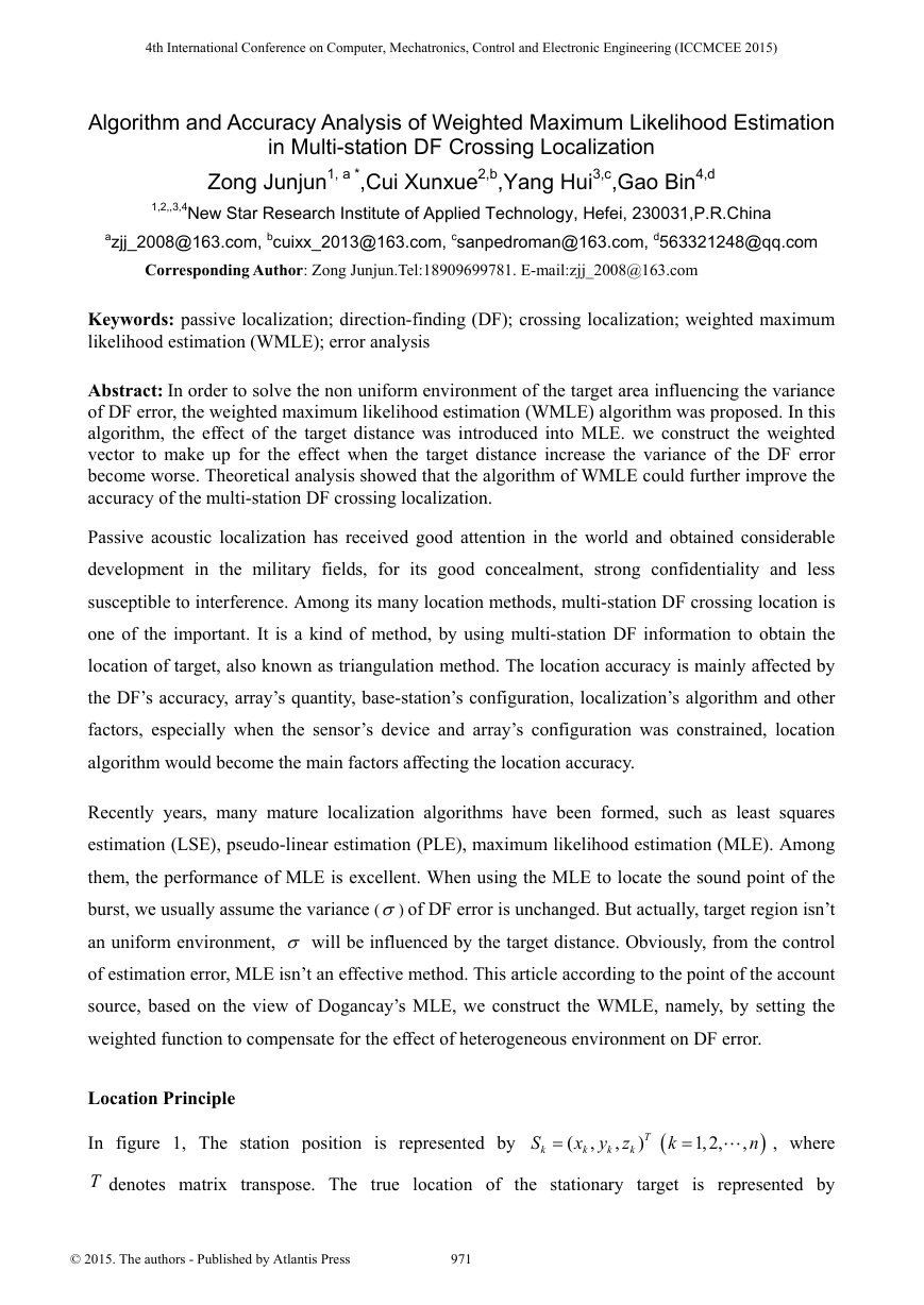Location Principle In figure 1, The station position is represented by =  , where 1,2, T denotes matrix transpose. The true location of the stationary target is represented by , x y z k )T , n = S k k k ) ( , ( k 4th International Conference on Computer, Mechatronics, Control and Electronic Engineering (ICCMCEE 2015) © 2015. The authors - Published by Atlantis Press971

( T ) p p p P , , z y x = X . We collect azimuth ( kθ ) and elevation ( kφ ) angle at each station. The unit of measurement is radian. It is assumed that azimuth and elevation angles are independent of each other, which satisfied with zero mean Gaussian noise, and their mean-square-deviation are denoted as kθσ and kφσ . Target ( , x y z , p p ) p z 1φ 1θ x y ( station1 , , x y z 1 1 1 ) z 2φ 2θ ( y x Nφ y station2 , , x y z 2 2 2 ) z Nθ Station n , x y z , n n n ( x ) Figure.1. 3-D AOA based source localization for noisy case According to the relations between stations and emitter sources, we can get equation (1) and (2) y x − − y )k x k θ k = 1 tan ( − φ k = 1 tan ( − （1） p 2 z ) x k − + z ( k y ) − y k p 2 ) （2） ( x p − ) ) ( ) = J ( ML p ( T e p W e p Weighted Maximum Likelihood Estimation According to the principle of maximum likelihood estimation, we can construct the maximum likelihood cost function 1 − Where W is a covariance matrix of the bearing noise and expressed as { 2 2 2 , , W diag σ σ σ σ σ σ  θ θ φ 1 2 n ) (    , e p p − θ θ φ φ  1 1 1 1 （3） ( e p is the error vector, which can be Therefore, the estimation value of the emitter source can be expressed as 2 2 2 , θ φ φ 1 2 n (  , p θ θ n n （4） ) p （5）  , φ φ n n   , = ) , − , − } ( , )  − = p   ( ( ) ) , , ˆ p ML = arg min p J ( p ) ML （6） The maximum likelihood location estimator is an nonlinear equation, so it does not have a closed-form solution and requires the use of a numerical search algorithm. The Gauss-Newton (GN) 972

algorithm, which is a batch iterative minimization technique, is often employed to calculate the MLE. The GN algorithm consists of X + = 1 i X i − ( J W J -1 T i i 1 − ) 1 − J W e P （7） T i i ( ) Where iJ is the 2N×3 Jacobian of ( ) e p − − − i i i i 0  0 J i ( ) i sin −  −  ˆ φ n ˆ θ 1 ˆ φ 1 ˆ φ 1 ( ) i ( ) i ( ) i ( ) i ( ) i                  sin ( )sin ( ) i ˆ ( )cos i θ n X S (8) ˆ cos φ 1 ˆ d 1 i  ˆ cos φ n ˆ d in ˆ i θ 1 X S ˆ sin φ 1 ˆ d 1 i  ˆ sin φ n ˆ d in ˆ sin ( )cos i θ 1 X S         =          Where ˆ d = ik k th station. coordinate of the target can be calculated by the PLE. From the above GN iterative, we can find the variance of DF error of azimuth ϕσ and elevation θσ is unchanging, but actually, DF error is influenced by the target distance, usually it will become big with the increase of the distance. Here, we assume that the variance of DF error of azimuth and elevation is σ when the distance is d , So we can draw iσ corresponding to the target distance id . The relationship can be expressed as ,denote as the distance between the i th emitter source and the is a 2×1 vector containing the first two entries of iX . The initial （9） 2 cos ˆ d 1 i  ˆ 2 cos θ n ˆ d in (1: 2) − 、 (1: 2) ˆ ( )sin i θ n X S X (1: 2) i iX (1: 2) S k kS ( ) i ˆ φ n sin ( ) i ( ) i − i − i − n n σ ϕ ki σ= ϕ k kid d kid d （10） σ θ ki σ= θ k The covariance matrix (W)of the DF error can be expressed as ,  2 , σ σ σ φ 2 2 θ ni 2 φ 1 i , , i , { 2 σ σ θ 2 2 θ 1 i , i =W i 2 , σ φ ni diag  } （11） Simulation Experiment Experiment Condition. Assuming the system is conformed by six base stations, which has uniform linear array and located at the x axis from -3000 to 3000. And the area of target is assumed as: axis x is ±3km, axis y is 1km～7km,axis z is ±0.5km. 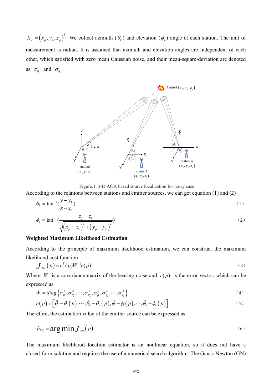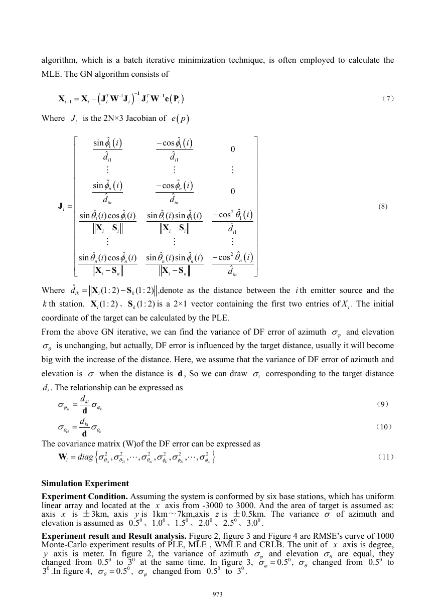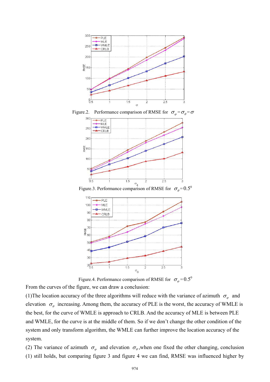The variance σ of azimuth and elevation is assumed as Experiment result and Result analysis. Figure 2, figure 3 and Figure 4 are RMSE’s curve of 1000 Monte-Carlo experiment results of PLE, MLE , WMLE and CRLB. The unit of x axis is degree, y axis is meter. In figure 2, the variance of azimuth ϕσ and elevation θσ are equal, they 00.5 to changed from 03 .In figure 4, 03 at the same time. In figure 3, 03 . , ϕσ changed from 00.5 、 01.0 、 01.5 、 02.0 、 02.5 、 03.0 . , θσ changed from 00.5 to 00.5 θσ = 00.5 to ϕσ = 00.5 973

Figure.2. Performance comparison of RMSE for ϕσ = θσ =σ Figure.3. Performance comparison of RMSE for θσ = 00.5 Figure.4. Performance comparison of RMSE for ϕσ = 00.5 From the curves of the figure, we can draw a conclusion: (1)The location accuracy of the three algorithms will reduce with the variance of azimuth ϕσ and elevation θσ increasing. Among them, the accuracy of PLE is the worst, the accuracy of WMLE is the best, for the curve of WMLE is approach to CRLB. And the accuracy of MLE is between PLE and WMLE, for the curve is at the middle of them. So if we don’t change the other condition of the system and only transform algorithm, the WMLE can further improve the location accuracy of the system. (2) The variance of azimuth ϕσ and elevation θσ ,when one fixed the other changing, conclusion (1) still holds, but comparing figure 3 and figure 4 we can find, RMSE was influenced higher by 974

ϕσ . Namely the location accuracy is influenced significantly higher by elevation DF error than azimuth DF error. Therefore, in condition of 3D, improving the accuracy of elevation angle is more helpful for multi-station DF crossing Location. Conclusion This paper studied the algorithm of the multi-station DF crossing localization. based on the MLE, the WMLE algorithm was proposed which considering the influence of the target distance. Experiment results show that the location accuracy of WMLE is much higher than that of PLE. which can make up of the error of the fixed variance and improve the influence of nonhomogeneous environment of the target area, compared with the MLE algorithm, WMLE can further improve the accuracy of the multi-station DF crossing localization. Acknowledgement This work was financially supported by the Fund of National Natural Science(61170252). References [1] Bishop,A.A.,Pathirana,P.N., A discussion on passive location discovery in emitter networks Using angle-only measurements. In proceedings of the 2006 International Wireless Communications and Mobile Computing Conference,Vancouver, BC,Canada(2006),p.1337 [3] Kostas E B,Max G,Lydia E K. Evaluation of Algorithms for Bearing-only SLAM[C]//Robotics and Automation(2006). ICRA 2006. in Proceedings of IEEE International Conference, Vol. 15-19 ( 2006), p.1937 [4] K.Dogancay,”3D passive localization in the presence of large bearing noise," in Proc.13th European Signal Processing Conference, EUSIPCO 2005, Antalya, Turkey, September 2005, in Press. [5] H.Hmam,K.Dogancay,”Passive localization of scanning emitters,” in proceeding of IEEE Transactions on aerospace and electronic systems, vol.46,no.2,pp.944-951,April 2010. [6] R.Badeau, B.David.”Weighted maximum likelihood autoregressive and moving average spectrum modeling,” in Proceeding of IEEE International Conference on Acoustics, Speech and Signal Processing(ICSAAP),2008,pp.3761-3764. 975