Towards End-to-End Speech Recognition
with Recurrent Neural Networks
Alex Graves
Google DeepMind, London, United Kingdom
Navdeep Jaitly
Department of Computer Science, University of Toronto, Canada
GRAVES@CS.TORONTO.EDU
NDJAITLY@CS.TORONTO.EDU
Abstract
This paper presents a speech recognition sys-
tem that directly transcribes audio data with text,
without requiring an intermediate phonetic repre-
sentation. The system is based on a combination
of the deep bidirectional LSTM recurrent neural
network architecture and the Connectionist Tem-
poral Classification objective function. A mod-
ification to the objective function is introduced
that trains the network to minimise the expec-
tation of an arbitrary transcription loss function.
This allows a direct optimisation of the word er-
ror rate, even in the absence of a lexicon or lan-
guage model. The system achieves a word error
rate of 27.3% on the Wall Street Journal corpus
with no prior linguistic information, 21.9% with
only a lexicon of allowed words, and 8.2% with a
trigram language model. Combining the network
with a baseline system further reduces the error
rate to 6.7%.
1. Introduction
Recent advances in algorithms and computer hardware
have made it possible to train neural networks in an end-
to-end fashion for tasks that previously required signifi-
cant human expertise. For example, convolutional neural
networks are now able to directly classify raw pixels into
high-level concepts such as object categories (Krizhevsky
et al., 2012) and messages on traffic signs (Ciresan et al.,
2011), without using hand-designed feature extraction al-
gorithms. Not only do such networks require less human
effort than traditional approaches, they generally deliver
superior performance. This is particularly true when very
large amounts of training data are available, as the bene-
Proceedings of the 31 st International Conference on Machine
Learning, Beijing, China, 2014. JMLR: W&CP volume 32. Copy-
right 2014 by the author(s).
fits of holistic optimisation tend to outweigh those of prior
knowledge.
While automatic speech recognition has greatly benefited
from the introduction of neural networks (Bourlard & Mor-
gan, 1993; Hinton et al., 2012), the networks are at present
only a single component in a complex pipeline. As with
traditional computer vision, the first stage of the pipeline
is input feature extraction: standard techniques include
mel-scale filterbanks (Davis & Mermelstein, 1980) (with
or without a further transform into Cepstral coefficients)
and speaker normalisation techniques such as vocal tract
length normalisation (Lee & Rose, 1998). Neural networks
are then trained to classify individual frames of acous-
tic data, and their output distributions are reformulated as
emission probabilities for a hidden Markov model (HMM).
The objective function used to train the networks is there-
fore substantially different from the true performance mea-
sure (sequence-level transcription accuracy). This is pre-
cisely the sort of inconsistency that end-to-end learning
seeks to avoid. In practice it is a source of frustration to
researchers, who find that a large gain in frame accuracy
can translate to a negligible improvement, or even deterio-
ration in transcription accuracy. An additional problem is
that the frame-level training targets must be inferred from
the alignments determined by the HMM. This leads to an
awkward iterative procedure, where network retraining is
alternated with HMM re-alignments to generate more accu-
rate targets. Full-sequence training methods such as Max-
imum Mutual Information have been used to directly train
HMM-neural network hybrids to maximise the probability
of the correct transcription (Bahl et al., 1986; Jaitly et al.,
2012). However these techniques are only suitable for re-
training a system already trained at frame-level, and require
the careful tuning of a large number of hyper-parameters—
typically even more than the tuning required for deep neu-
ral networks.
While the transcriptions used to train speech recognition
systems are lexical, the targets presented to the networks
�
Towards End-to-End Speech Recognition with Recurrent Neural Networks
are usually phonetic. A pronunciation dictionary is there-
fore needed to map from words to phoneme sequences.
Creating such dictionaries requires significant human effort
and often proves critical to overall performance. A further
complication is that, because multi-phone contextual mod-
els are used to account for co-articulation effects, ‘state
tying’ is needed to reduce the number of target classes—
another source of expert knowledge. Lexical states such as
graphemes and characters have been considered for HMM-
based recognisers as a way of dealing with out of vocabu-
lary (OOV) words (Galescu, 2003; Bisani & Ney, 2005),
however they were used to augment rather than replace
phonetic models.
Finally, the acoustic scores produced by the HMM are
combined with a language model trained on a text cor-
pus. In general the language model contains a great deal
of prior information, and has a huge impact on perfor-
mance. Modelling language separately from sound is per-
haps the most justifiable departure from end-to-end learn-
ing, since it is easier to learn linguistic dependencies from
text than speech, and arguable that literate humans do the
same thing. Nonetheless, with the advent of speech corpora
containing tens of thousands of hours of labelled data, it
may be possible to learn the language model directly from
the transcripts.
The goal of this paper is a system where as much of the
speech pipeline as possible is replaced by a single recur-
rent neural network (RNN) architecture. Although it is
possible to directly transcribe raw speech waveforms with
RNNs (Graves, 2012, Chapter 9) or features learned with
restricted Boltzmann machines (Jaitly & Hinton, 2011),
the computational cost is high and performance tends to be
worse than conventional preprocessing. We have therefore
chosen spectrograms as a minimal preprocessing scheme.
The spectrograms are processed by a deep bidirectional
LSTM network (Graves et al., 2013) with a Connectionist
Temporal Classification (CTC) output layer (Graves et al.,
2006; Graves, 2012, Chapter 7). The network is trained
directly on the text transcripts: no phonetic representation
(and hence no pronunciation dictionary or state tying) is
used. Furthermore, since CTC integrates out over all pos-
sible input-output alignments, no forced alignment is re-
quired to provide training targets. The combination of bidi-
rectional LSTM and CTC has been applied to character-
level speech recognition before (Eyben et al., 2009), how-
ever the relatively shallow architecture used in that work
did not deliver compelling results (the best character error
rate was almost 20%).
The basic system is enhanced by a new objective function
that trains the network to directly optimise the word error
rate.
Experiments on the Wall Street Journal speech corpus
demonstrate that the system is able to recognise words to
reasonable accuracy, even in the absence of a language
model or dictionary, and that when combined with a lan-
guage model it performs comparably to a state-of-the-art
pipeline.
2. Network Architecture
Given an input sequence x = (x1, . . . , xT ), a standard re-
current neural network (RNN) computes the hidden vector
sequence h = (h1, . . . , hT ) and output vector sequence
y = (y1, . . . , yT ) by iterating the following equations from
t = 1 to T :
ht = H (Wihxt + Whhht−1 + bh)
yt = Whoht + bo
(1)
(2)
where the W terms denote weight matrices (e.g. Wih is
the input-hidden weight matrix), the b terms denote bias
vectors (e.g. bh is hidden bias vector) and H is the hidden
layer activation function.
H is usually an elementwise application of a sigmoid func-
tion. However we have found that the Long Short-Term
Memory (LSTM) architecture (Hochreiter & Schmidhuber,
1997), which uses purpose-built memory cells to store in-
formation, is better at finding and exploiting long range
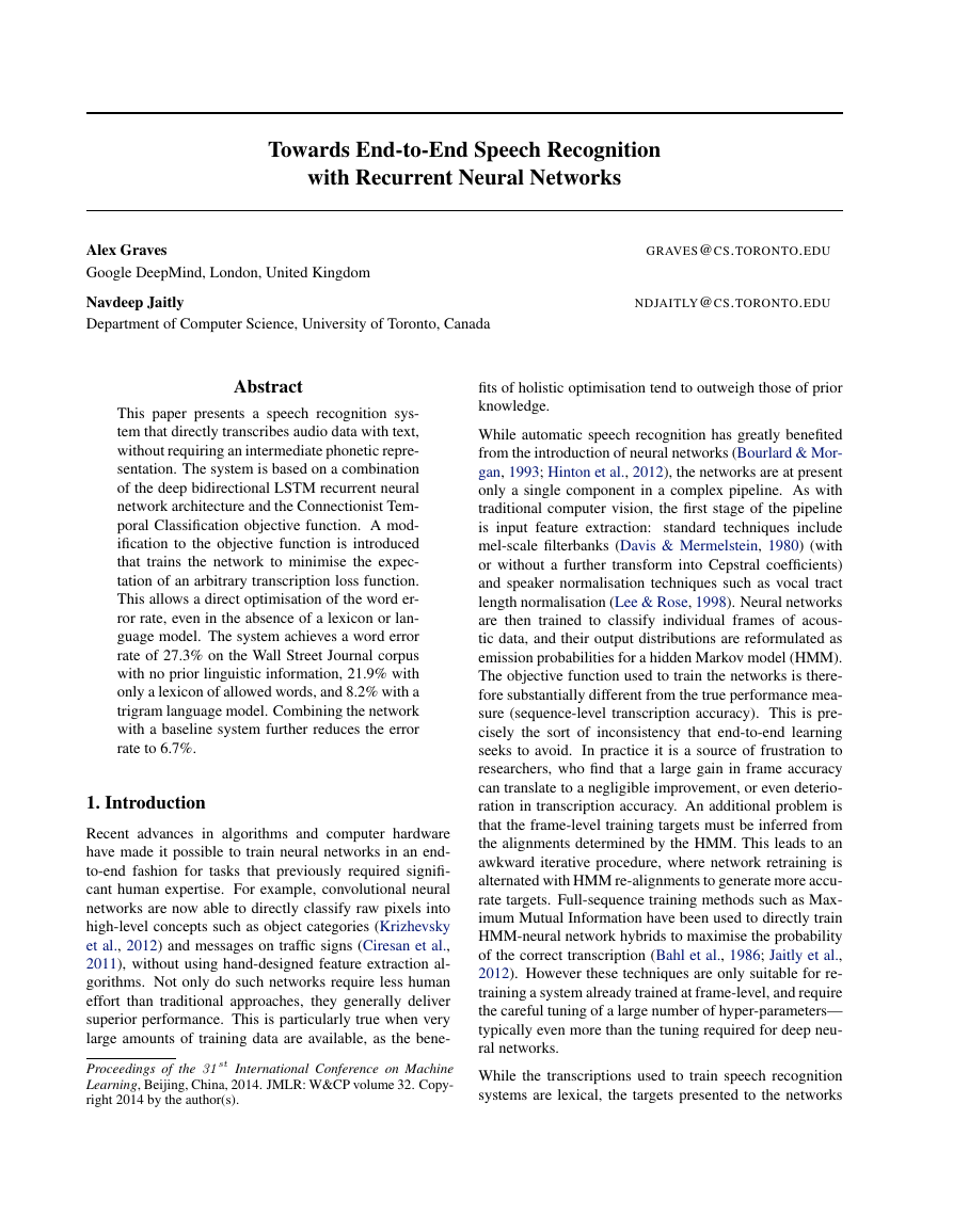
context. Fig. 1 illustrates a single LSTM memory cell. For
the version of LSTM used in this paper (Gers et al., 2002)
H is implemented by the following composite function:
it = σ (Wxixt + Whiht−1 + Wcict−1 + bi)
ft = σ (Wxf xt + Whf ht−1 + Wcf ct−1 + bf )
ct = ftct−1 + it tanh (Wxcxt + Whcht−1 + bc)
ot = σ (Wxoxt + Whoht−1 + Wcoct + bo)
ht = ot tanh(ct)
(3)
(4)
(5)
(6)
(7)
where σ is the logistic sigmoid function, and i, f, o and
c are respectively the input gate, forget gate, output gate
and cell activation vectors, all of which are the same size
as the hidden vector h. The weight matrix subscripts have
the obvious meaning, for example Whi is the hidden-input
gate matrix, Wxo is the input-output gate matrix etc. The
weight matrices from the cell to gate vectors (e.g. Wci) are
diagonal, so element m in each gate vector only receives
input from element m of the cell vector. The bias terms
(which are added to i, f, c and o) have been omitted for
clarity.
One shortcoming of conventional RNNs is that they are
only able to make use of previous context. In speech recog-
nition, where whole utterances are transcribed at once,
there is no reason not to exploit future context as well.
Bidirectional RNNs (BRNNs) (Schuster & Paliwal, 1997)
�
Towards End-to-End Speech Recognition with Recurrent Neural Networks
Figure 1. Long Short-term Memory Cell.
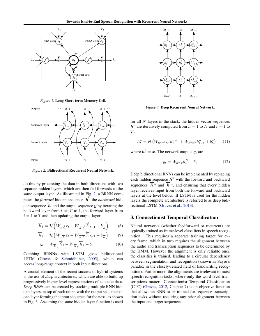
Figure 3. Deep Recurrent Neural Network.
for all N layers in the stack, the hidden vector sequences
hn are iteratively computed from n = 1 to N and t = 1 to
T :
t = HWhn−1hn hn−1
hn
t + Whnhn hn
t−1 + bn
h
where h0 = x. The network outputs yt are
yt = WhN yhN
t + bo
(11)
(12)
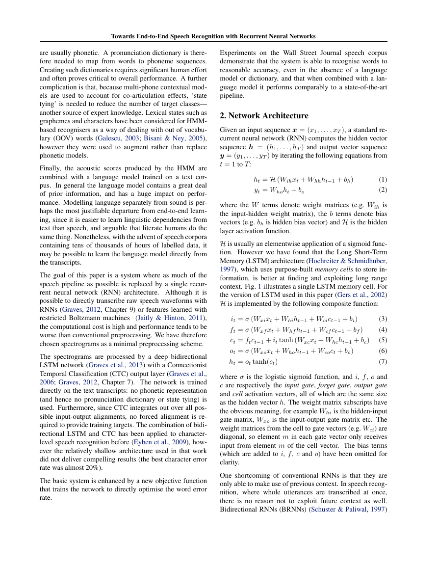
Figure 2. Bidirectional Recurrent Neural Network.
do this by processing the data in both directions with two
separate hidden layers, which are then fed forwards to the
same output layer. As illustrated in Fig. 2, a BRNN com-
−→
putes the forward hidden sequence
h , the backward hid-
←−
h and the output sequence y by iterating the
den sequence
backward layer from t = T to 1, the forward layer from
t = 1 to T and then updating the output layer:
h t = H
h t = H
−→
←−
yt = W−→
h y
−→
h t−1 + b−→
←−
h t+1 + b←−
h
h
h
W
xt + W−→
−→
h
x
←−
W
h
−→
h t + W←−
−→
h
xt + W←−
←−
h
←−
h t + bo
h
x
h y
(8)
(9)
(10)
Combing BRNNs with LSTM gives
bidirectional
LSTM (Graves & Schmidhuber, 2005), which can
access long-range context in both input directions.
A crucial element of the recent success of hybrid systems
is the use of deep architectures, which are able to build up
progressively higher level representations of acoustic data.
Deep RNNs can be created by stacking multiple RNN hid-
den layers on top of each other, with the output sequence of
one layer forming the input sequence for the next, as shown
in Fig. 3. Assuming the same hidden layer function is used
−→
h n and
Deep bidirectional RNNs can be implemented by replacing
each hidden sequence hn with the forward and backward
←−
sequences
h n, and ensuring that every hidden
layer receives input from both the forward and backward
layers at the level below. If LSTM is used for the hidden
layers the complete architecture is referred to as deep bidi-
rectional LSTM (Graves et al., 2013).
3. Connectionist Temporal Classification
Neural networks (whether feedforward or recurrent) are
typically trained as frame-level classifiers in speech recog-
nition. This requires a separate training target for ev-
ery frame, which in turn requires the alignment between
the audio and transcription sequences to be determined by
the HMM. However the alignment is only reliable once
the classifier is trained, leading to a circular dependency
between segmentation and recognition (known as Sayre’s
paradox in the closely-related field of handwriting recog-
nition). Furthermore, the alignments are irrelevant to most
speech recognition tasks, where only the word-level tran-
scriptions matter. Connectionist Temporal Classification
(CTC) (Graves, 2012, Chapter 7) is an objective function
that allows an RNN to be trained for sequence transcrip-
tion tasks without requiring any prior alignment between
the input and target sequences.
�
Towards End-to-End Speech Recognition with Recurrent Neural Networks
The output layer contains a single unit for each of the tran-
scription labels (characters, phonemes, musical notes etc.),
plus an extra unit referred to as the ‘blank’ which corre-
sponds to a null emission. Given a length T input sequence
x, the output vectors yt are normalised with the softmax
function, then interpreted as the probability of emitting the
label (or blank) with index k at time t:
Pr(k, t|x) =
(13)
expyk
k expyk
t
t
where yk
t is element k of yt. A CTC alignment a is a length
T sequence of blank and label indices. The probability
Pr(a|x) of a is the product of the emission probabilities
at every time-step:
Pr(a|x) =
Pr(at, t|x)
(14)
T
t=1
For a given transcription sequence, there are as many possi-
ble alignments as there different ways of separating the la-
bels with blanks. For example (using ‘−’ to denote blanks)
the alignments (a,−, b, c,−,−) and (−,−, a,−, b, c) both
correspond to the transcription (a, b, c). When the same
label appears on successive time-steps in an alignment,
the repeats are removed:
therefore (a, b, b, b, c, c) and
(a,−, b,−, c, c) also correspond to (a, b, c). Denoting by
B an operator that removes first the repeated labels, then
the blanks from alignments, and observing that the total
probability of an output transcription y is equal to the sum
of the probabilities of the alignments corresponding to it,
we can write
Pr(y|x) =
Pr(a|x)
(15)
a∈B−1(y)
This ‘integrating out’ over possible alignments is what al-
lows the network to be trained with unsegmented data. The
intuition is that, because we don’t know where the labels
within a particular transcription will occur, we sum over
all the places where they could occur. Eq. (15) can be ef-
ficiently evaluated and differentiated using a dynamic pro-
gramming algorithm (Graves et al., 2006). Given a target
transcription y∗, the network can then be trained to min-
imise the CTC objective function:
CT C(x) = − log Pr(y∗|x)
(16)
4. Expected Transcription Loss
The CTC objective function maximises the log probabil-
ity of getting the sequence transcription completely correct.
The relative probabilities of the incorrect transcriptions are
therefore ignored, which implies that they are all equally
bad. In most cases however, transcription performance is
assessed in a more nuanced way.
In speech recognition,
for example, the standard measure is the word error rate
(WER), defined as the edit distance between the true word
sequence and the most probable word sequence emitted by
the transcriber. We would therefore prefer transcriptions
with high WER to be more probable than those with low
WER. In the interest of reducing the gap between the ob-
jective function and the test criteria, this section proposes
a method that allows an RNN to be trained to optimise the
expected value of an arbitrary loss function defined over
output transcriptions (such as WER).
The network structure and the interpretation of the output
activations as the probability of emitting a label (or blank)
at a particular time-step, remain the same as for CTC.
Given input sequence x, the distribution Pr(y|x) over tran-
scriptions sequences y defined by CTC, and a real-valued
transcription loss function L(x, y), the expected transcrip-
tion loss L(x) is defined as
L(x) =
Pr(y|x)L(x, y)
(17)
In general we will not be able to calculate this expectation
exactly, and will instead use Monte-Carlo sampling to ap-
proximate both L and its gradient. Substituting Eq. (15)
into Eq. (17) we see that
y
Eq. (14) shows that samples can be drawn from Pr(a|x)
by independently picking from Pr(k, t|x) at each time-step
and concatenating the results, making it straightforward to
approximate the loss:
L(x) ≈ 1
N
L(x,B(ai)), ai ∼ Pr(a|x)
(20)
To differentiate L with respect to the network outputs, first
observe from Eq. (13) that
N
i=1
∂ log P r(a|x)
∂ Pr(k, t|x)
Then substitute into Eq.
∇xf (x) = f (x)∇x log f (x), to yield:
=
δatk
Pr(k, t|x)
(19), applying the identity
(21)
a
a
=
=
=
a:at=k
∂ Pr(a|x)
∂ Pr(k, t|x)
Pr(a|x)
L(x,B(a))
∂ log Pr(a|x)
∂ Pr(k, t|x)
L(x,B(a))
Pr(a|x, at = k)L(x,B(a))
∂L(x)
∂ Pr(k, t|x)
y
a
L(x) =
=
Pr(a|x)L(x, y)
a∈B−1(y)
Pr(a|x)L(x,B(a))
(18)
(19)
�
Towards End-to-End Speech Recognition with Recurrent Neural Networks
This expectation can also be approximated with Monte-
Carlo sampling. Because the output probabilities are in-
dependent, an unbiased sample ai from Pr(a|x) can be
converted to an unbiased sample from Pr(a|x, at = k) by
setting ai
t = k. Every ai can therefore be used to provide
a gradient estimate for every Pr(k, t|x) as follows:
∂L(x)
∂ Pr(k, t|x)
≈ 1
N
N
i=1
L(x,B(ai,t,k))
(22)
t
t = ai
t∀t = t, ai,t,k
with ai ∼ Pr(a|x) and ai,t,k
= k.
The advantage of reusing the alignment samples (as op-
posed to picking separate alignments for every k, t) is that
the noise due to the loss variance largely cancels out, and
only the difference in loss due to altering individual labels is
added to the gradient. As has been widely discussed in the
policy gradients literature and elsewhere (Peters & Schaal,
2008), noise minimisation is crucial when optimising with
stochastic gradient estimates. The Pr(k, t|x) derivatives
are passed through the softmax function to give:
L(x,B(ai)) − Z(ai, t)
N
i=1
∂L(x)
∂yk
t
where
N
≈ Pr(k, t|x)
Z(ai, t) =
Pr(k, t|x)L(x,B(ai,t,k
))
k
t by a given ai is therefore equal
The derivative added to yk
t = k, and the ex-
to the difference between the loss with ai
t sampled from Pr(k, t|x). This means
pected loss with ai
the network only receives an error term for changes to
the alignment that alter the loss. For example, if the loss
function is the word error rate and the sampled alignment
yields the character transcription “WTRD ERROR RATE”
the gradient would encourage outputs changing the second
output label to ‘O’, discourage outputs making changes to
the other two words and be close to zero everywhere else.
For the sampling procedure to be effective, there must be
a reasonable probability of picking alignments whose vari-
ants receive different losses. The vast majority of align-
ments drawn from a randomly initialised network will give
completely wrong transcriptions, and there will therefore
be little chance of altering the loss by modifying a single
output. We therefore recommend that expected loss min-
imisation is used to retrain a network already trained with
CTC, rather than applied from the start.
Sampling alignments is cheap, so the only significant com-
putational cost in the procedure is recalculating the loss
for the alignment variants. However, for many loss func-
tions (including word error rate) this could be optimised by
only recalculating that part of the loss corresponding to the
alignment change. For our experiments, five samples per
sequence gave sufficiently low variance gradient estimates
for effective training.
Note that, in order to calculate the word error rate, an end-
of-word label must be used as a delimiter.
5. Decoding
Decoding a CTC network (that is, finding the most prob-
able output transcription y for a given input sequence x)
can be done to a first approximation by picking the single
most probable output at every timestep and returning the
corresponding transcription:
argmaxy Pr(y|x) ≈ B (argmaxa Pr(a|x))
More accurate decoding can be performed with a beam
search algorithm, which also makes it possible to integrate
a language model. The algorithm is similar to decoding
methods used for HMM-based systems, but differs slightly
due to the changed interpretation of the network outputs.
In a hybrid system the network outputs are interpreted as
posterior probabilities of state occupancy, which are then
combined with transition probabilities provided by a lan-
guage model and an HMM. With CTC the network out-
puts themselves represent transition probabilities (in HMM
terms, the label activations are the probability of making
transitions into different states, and the blank activation is
the probability of remaining in the current state). The situa-
tion is further complicated by the removal of repeated label
emissions on successive time-steps, which makes it nec-
essary to distinguish alignments ending with blanks from
those ending with labels.
The pseudocode in Algorithm 1 describes a simple beam
search procedure for a CTC network, which allows the
integration of a dictionary and language model. De-
fine Pr−(y, t), Pr+(y, t) and Pr(y, t) respectively as the
blank, non-blank and total probabilities assigned to some
(partial) output transcription y, at time t by the beam
search, and set Pr(y, t) = Pr−(y, t) + Pr+(y, t). Define
the extension probability Pr(k, y, t) of y by label k at time
t as follows:
Pr(k, y, t) = Pr(k, t|x) Pr(k|y)
Pr−(y, t − 1) if ye = k
Pr(y, t − 1) otherwise
where Pr(k, t|x) is the CTC emission probability of k at t,
as defined in Eq. (13), Pr(k|y) is the transition probability
from y to y + k and ye is the final label in y. Lastly, define
ˆy as the prefix of y with the last label removed, and ∅ as
the empty sequence, noting that Pr+(∅, t) = 0 ∀t.
The transition probabilities Pr(k|y) can be used to inte-
grate prior linguistic information into the search.
If no
�
Towards End-to-End Speech Recognition with Recurrent Neural Networks
Algorithm 1 CTC Beam Search
Initalise: B ← {∅}; Pr−(∅, 0) ← 1
for t = 1 . . . T do
ˆB ← the W most probable sequences in B
B ← {}
for y ∈ ˆB do
if y = ∅ then
Pr+(y, t) ← Pr+(y, t − 1) Pr(ye, t|x)
if ˆy ∈ ˆB then
Pr+(y, t) ← Pr+(y, t) + Pr(ye, ˆy, t)
Pr−(y, t) ← Pr(y, t − 1) Pr(−, t|x)
Add y to B
for k = 1 . . . K do
Pr−(y + k, t) ← 0
Pr+(y + k, t) ← Pr(k, y, t)
Add (y + k) to B
Return: maxy∈B Pr
1|y| (y, T )
such knowledge is present (as with standard CTC) then all
Pr(k|y) are set to 1. Constraining the search to dictionary
words can be easily implemented by setting Pr(k|y) = 1 if
(y + k) is in the dictionary and 0 otherwise. To apply a sta-
tistical language model, note that Pr(k|y) should represent
normalised label-to-label transition probabilities. To con-
vert a word-level language model to a label-level one, first
note that any label sequence y can be expressed as the con-
catenation y = (w + p) where w is the longest complete
sequence of dictionary words in y and p is the remaining
word prefix. Both w and p may be empty. Then we can
write
w∈(p+k)∗ Prγ(w|w)
w∈p∗ Prγ(w|w)
Pr(k|y) =
(23)
where Pr(w|w) is the probability assigned to the transition
from the word history w to the word w, p∗ is the set of
dictionary words prefixed by p and γ is the language model
weighting factor.
The length normalisation in the final step of the algo-
rithm is helpful when decoding with a language model,
as otherwise sequences with fewer transitions are unfairly
favoured; it has little impact otherwise.
6. Experiments
The experiments were carried out on the Wall Street Jour-
nal (WSJ) corpus (available as LDC corpus LDC93S6B
and LDC94S13B). The RNN was trained on both the 14
hour subset ‘train-si84’ and the full 81 hour set, with the
‘test-dev93’ development set used for validation. For both
training sets, the RNN was trained with CTC, as described
in Section 3, using the characters in the transcripts as the
target sequences. The RNN was then retrained to minimise
the expected word error rate using the method from Sec-
tion 4, with five alignment samples per sequence.
There were a total of 43 characters (including upper case
letters, punctuation and a space character to delimit the
words). The input data were presented as spectrograms de-
rived from the raw audio files using the ‘specgram’ function
of the ‘matplotlib’ python toolkit, with width 254 Fourier
windows and an overlap of 127 frames, giving 128 inputs
per frame.
The network had five levels of bidirectional LSTM hid-
den layers, with 500 cells in each layer, giving a total of
∼ 26.5M weights. It was trained using stochastic gradient
descent with one weight update per utterance, a learning
rate of 10−4 and a momentum of 0.9.
The RNN was compared to a baseline deep neural network-
HMM hybrid (DNN-HMM). The DNN-HMM was created
using alignments from an SGMM-HMM system trained us-
ing Kaldi recipe ‘s5’, model ‘tri4b’(Povey et al., 2011).
The 14 hour subset was first used to train a Deep Belief
Network (DBN) (Hinton & Salakhutdinov, 2006) with six
hidden layers of 2000 units each. The input was 15 frames
of Mel-scale log filterbanks (1 centre frame ±7 frames of
context) with 40 coefficients, deltas and accelerations. The
DBN was trained layerwise then used to initialise a DNN.
The DNN was trained to classify the central input frame
into one of 3385 triphone states. The DNN was trained with
stochastic gradient descent, starting with a learning rate of
0.1, and momentum of 0.9. The learning rate was divided
by two at the end of each epoch which failed to reduce the
frame error rate on the development set. After six failed at-
tempts, the learning rate was frozen. The DNN posteriors
were divided by the square root of the state priors during
decoding.
The RNN was first decoded with no dictionary or language
model, using the space character to segment the charac-
ter outputs into words, and thereby calculate the WER.
The network was then decoded with a 146K word dictio-
nary, followed by monogram, bigram and trigram language
models. The dictionary was built by extending the default
WSJ dictionary with 125K words using some augmen-
tation rules implemented into the Kaldi recipe ‘s5’. The
languge models were built on this extended dictionary, us-
ing data from the WSJ CD (see scripts ‘wsj extend dict.sh’
and ‘wsj train lms.sh’ in recipe ‘s5’). The language model
weight was optimised separately for all experiments. For
the RNN experiments with no linguistic information, and
those with only a dictionary, the beam search algorithm in
Section 5 was used for decoding. For the RNN experiments
with a language model, an alternative method was used,
partly due to implementation difficulties and partly to en-
sure a fair comparison with the baseline system: an N-best
list of at most 300 candidate transcriptions was extracted
from the baseline DNN-HMM and rescored by the RNN
using Eq. (16). The RNN scores were then combined with
�
Towards End-to-End Speech Recognition with Recurrent Neural Networks
Table 1. Wall Street Journal Results. All scores are word er-
ror rate/character error rate (where known) on the evaluation set.
‘LM’ is the Language model used for decoding. ‘14 Hr’ and ‘81
Hr’ refer to the amount of data used for training.
SYSTEM
RNN-CTC
RNN-CTC
RNN-CTC
RNN-CTC
RNN-CTC
RNN-WER
RNN-WER
RNN-WER
RNN-WER
RNN-WER
BASELINE
BASELINE
BASELINE
BASELINE
BASELINE
COMBINATION
LM
NONE
DICTIONARY
MONOGRAM
BIGRAM
TRIGRAM
NONE
DICTIONARY
MONOGRAM
BIGRAM
TRIGRAM
NONE
DICTIONARY
MONOGRAM
BIGRAM
TRIGRAM
TRIGRAM
14 HR
74.2/30.9
69.2/30.0
25.8
15.5
13.5
74.5/31.3
69.7/31.0
26.0
15.3
13.5
—
56.1
23.4
11.6
9.4
—
81 HR
30.1/9.2
24.0/8.0
15.8
10.4
8.7
27.3/8.4
21.9/7.3
15.2
9.8
8.2
—
51.1
19.9
9.4
7.8
6.7
the language model to rerank the N-best lists and the WER
of the best resulting transcripts was recorded. The best re-
sults were obtained with an RNN score weight of 7.7 and a
language model weight of 16.
For the 81 hour training set, the oracle error rates for the
monogram, bigram and trigram candidates were 8.9%, 2%
and 1.4% resepectively, while the anti-oracle (rank 300) er-
ror rates varied from 45.5% for monograms and 33% for
trigrams. Using larger N-best lists (up to N=1000) did not
yield significant performance improvements, from which
we concluded that the list was large enough to approximate
the true decoding performance of the RNN.
An additional experiment was performed to measure the ef-
fect of combining the RNN and DNN. The candidate scores
for ‘RNN-WER’ trained on the 81 hour set were blended
with the DNN acoustic model scores and used to rerank
the candidates. Best results were obtained with a language
model weight of 11, an RNN score weight of 1 and a DNN
weight of 1.
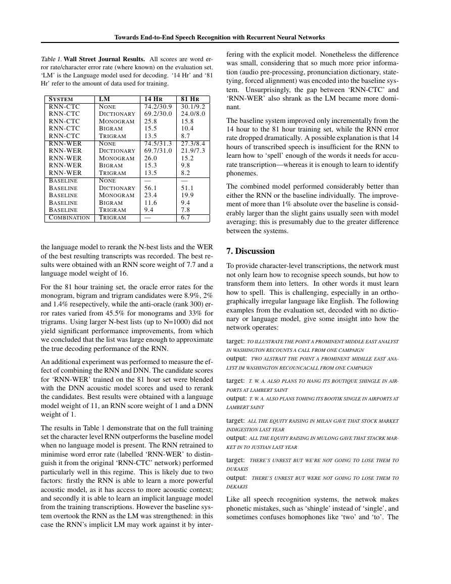
The results in Table 1 demonstrate that on the full training
set the character level RNN outperforms the baseline model
when no language model is present. The RNN retrained to
minimise word error rate (labelled ‘RNN-WER’ to distin-
guish it from the original ‘RNN-CTC’ network) performed
particularly well in this regime. This is likely due to two
factors: firstly the RNN is able to learn a more powerful
acoustic model, as it has access to more acoustic context;
and secondly it is able to learn an implicit language model
from the training transcriptions. However the baseline sys-
tem overtook the RNN as the LM was strengthened: in this
case the RNN’s implicit LM may work against it by inter-
fering with the explicit model. Nonetheless the difference
was small, considering that so much more prior informa-
tion (audio pre-processing, pronunciation dictionary, state-
tying, forced alignment) was encoded into the baseline sys-
tem. Unsurprisingly, the gap between ‘RNN-CTC’ and
‘RNN-WER’ also shrank as the LM became more domi-
nant.
The baseline system improved only incrementally from the
14 hour to the 81 hour training set, while the RNN error
rate dropped dramatically. A possible explanation is that 14
hours of transcribed speech is insufficient for the RNN to
learn how to ‘spell’ enough of the words it needs for accu-
rate transcription—whereas it is enough to learn to identify
phonemes.
The combined model performed considerably better than
either the RNN or the baseline individually. The improve-
ment of more than 1% absolute over the baseline is consid-
erably larger than the slight gains usually seen with model
averaging; this is presumably due to the greater difference
between the systems.
7. Discussion
To provide character-level transcriptions, the network must
not only learn how to recognise speech sounds, but how to
transform them into letters. In other words it must learn
how to spell. This is challenging, especially in an ortho-
graphically irregular language like English. The following
examples from the evaluation set, decoded with no dictio-
nary or language model, give some insight into how the
network operates:
target: TO ILLUSTRATE THE POINT A PROMINENT MIDDLE EAST ANALYST
IN WASHINGTON RECOUNTS A CALL FROM ONE CAMPAIGN
output: TWO ALSTRAIT THE POINT A PROMINENT MIDILLE EAST ANA-
LYST IM WASHINGTON RECOUNCACALL FROM ONE CAMPAIGN
target: T. W. A. ALSO PLANS TO HANG ITS BOUTIQUE SHINGLE IN AIR-
PORTS AT LAMBERT SAINT
output: T. W. A. ALSO PLANS TOHING ITS BOOTIK SINGLE IN AIRPORTS AT
LAMBERT SAINT
target: ALL THE EQUITY RAISING IN MILAN GAVE THAT STOCK MARKET
INDIGESTION LAST YEAR
output: ALL THE EQUITY RAISING IN MULONG GAVE THAT STACRK MAR-
KET IN TO JUSTIAN LAST YEAR
target: THERE’S UNREST BUT WE’RE NOT GOING TO LOSE THEM TO
DUKAKIS
output: THERE’S UNREST BUT WERE NOT GOING TO LOSE THEM TO
DEKAKIS
Like all speech recognition systems, the netwok makes
phonetic mistakes, such as ‘shingle’ instead of ‘single’, and
sometimes confuses homophones like ‘two’ and ‘to’. The
�
Towards End-to-End Speech Recognition with Recurrent Neural Networks
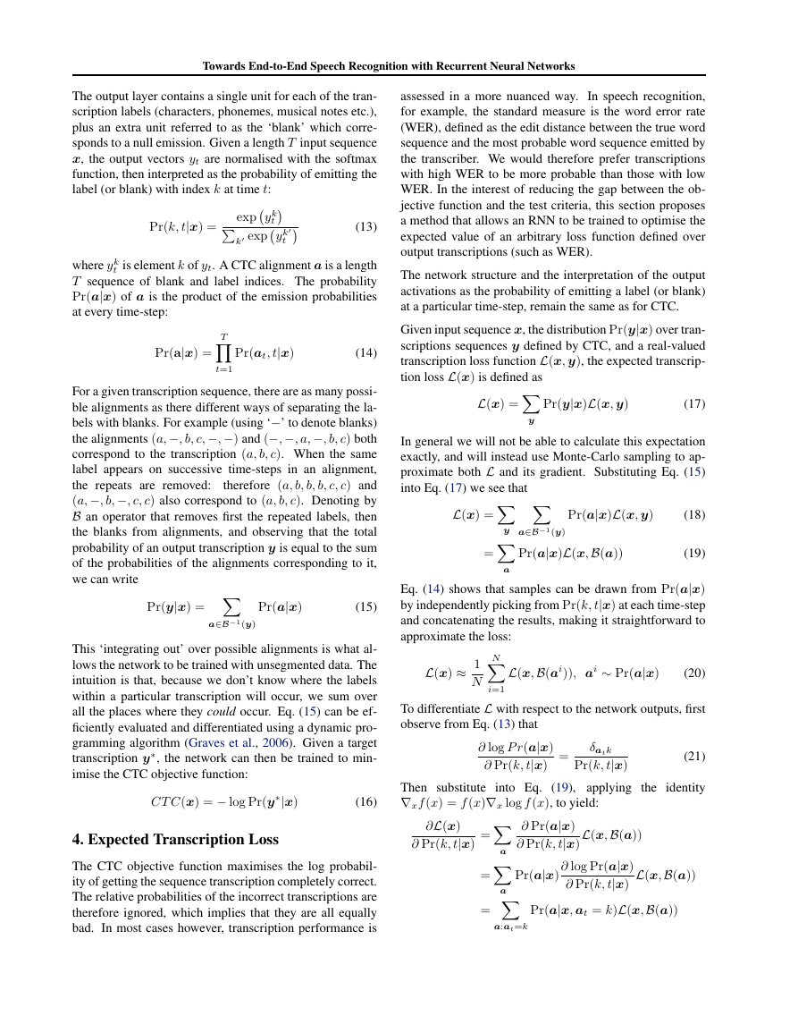
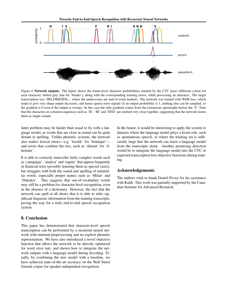
Figure 4. Network outputs. The figure shows the frame-level character probabilities emitted by the CTC layer (different colour for
each character, dotted grey line for ‘blanks’), along with the corresponding training errors, while processing an utterance. The target
transcription was ‘HIS FRIENDS ’, where the underscores are end-of-word markers. The network was trained with WER loss, which
tends to give very sharp output decisions, and hence sparse error signals (if an output probability is 1, nothing else can be sampled, so
the gradient is 0 even if the output is wrong). In this case the only gradient comes from the extraneous apostrophe before the ‘S’. Note
that the characters in common sequences such as ‘IS’, ‘RI’ and ‘END’ are emitted very close together, suggesting that the network learns
them as single sounds.
In the future, it would be interesting to apply the system to
datasets where the language model plays a lesser role, such
as spontaneous speech, or where the training set is suffi-
ciently large that the network can learn a language model
from the transcripts alone. Another promising direction
would be to integrate the language model into the CTC or
expected transcription loss objective functions during train-
ing.
Acknowledgements
The authors wish to thank Daniel Povey for his assistance
with Kaldi. This work was partially supported by the Cana-
dian Institute for Advanced Research.
latter problem may be harder than usual to fix with a lan-
guage model, as words that are close in sound can be quite
distant in spelling. Unlike phonetic systems, the network
also makes lexical errors—e.g. ‘bootik’ for ‘boutique’—
and errors that combine the two, such as ‘alstrait’ for ‘il-
lustrate’.
It is able to correctly transcribe fairly complex words such
as ‘campaign’, ‘analyst’ and ‘equity’ that appear frequently
in financial texts (possibly learning them as special cases),
but struggles with both the sound and spelling of unfamil-
iar words, especially proper names such as ‘Milan’ and
‘Dukakis’. This suggests that out-of-vocabulary words
may still be a problem for character-level recognition, even
in the absence of a dictionary. However, the fact that the
network can spell at all shows that it is able to infer sig-
nificant linguistic information from the training transcripts,
paving the way for a truly end-to-end speech recognition
system.
8. Conclusion
This paper has demonstrated that character-level speech
transcription can be performed by a recurrent neural net-
work with minimal preprocessing and no explicit phonetic
representation. We have also introduced a novel objective
function that allows the network to be directly optimised
for word error rate, and shown how to integrate the net-
work outputs with a language model during decoding. Fi-
nally, by combining the new model with a baseline, we
have achieved state-of-the-art accuracy on the Wall Street
Journal corpus for speaker independent recognition.
01probabilityHISFRIE_ND'S_outputswaveformerrors�



 2023年江西萍乡中考道德与法治真题及答案.doc
 2012年重庆南川中考生物真题及答案.doc
 2013年江西师范大学地理学综合及文艺理论基础考研真题.doc
 2020年四川甘孜小升初语文真题及答案I卷.doc
 2020年注册岩土工程师专业基础考试真题及答案.doc
 2023-2024学年福建省厦门市九年级上学期数学月考试题及答案.doc
 2021-2022学年辽宁省沈阳市大东区九年级上学期语文期末试题及答案.doc
 2022-2023学年北京东城区初三第一学期物理期末试卷及答案.doc
 2018上半年江西教师资格初中地理学科知识与教学能力真题及答案.doc
 2012年河北国家公务员申论考试真题及答案-省级.doc
 2020-2021学年江苏省扬州市江都区邵樊片九年级上学期数学第一次质量检测试题及答案.doc
 2022下半年黑龙江教师资格证中学综合素质真题及答案.doc