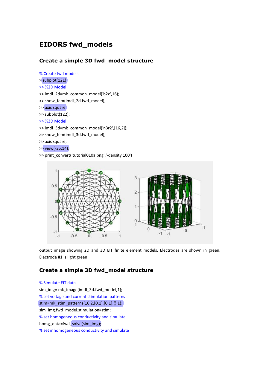
EIDORS fwd_models
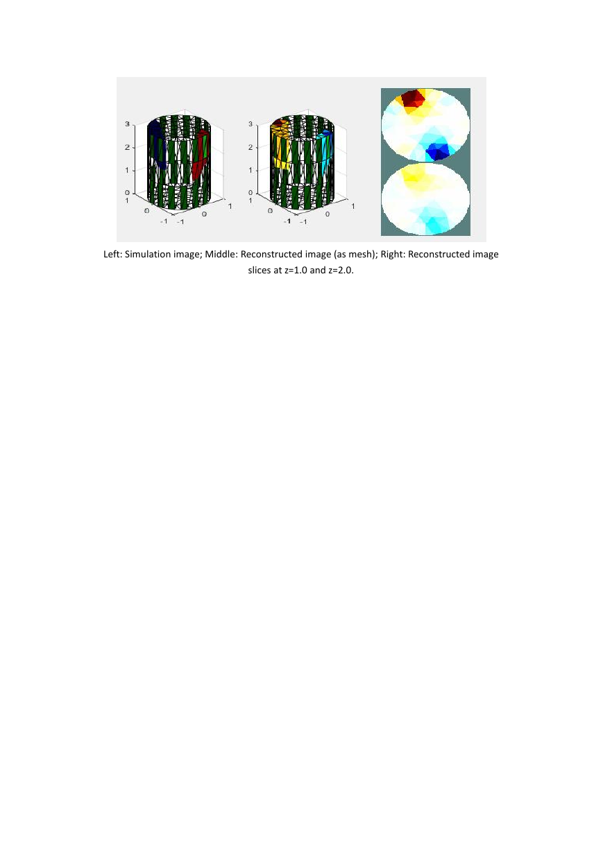
Create a simple 3D fwd_model structure
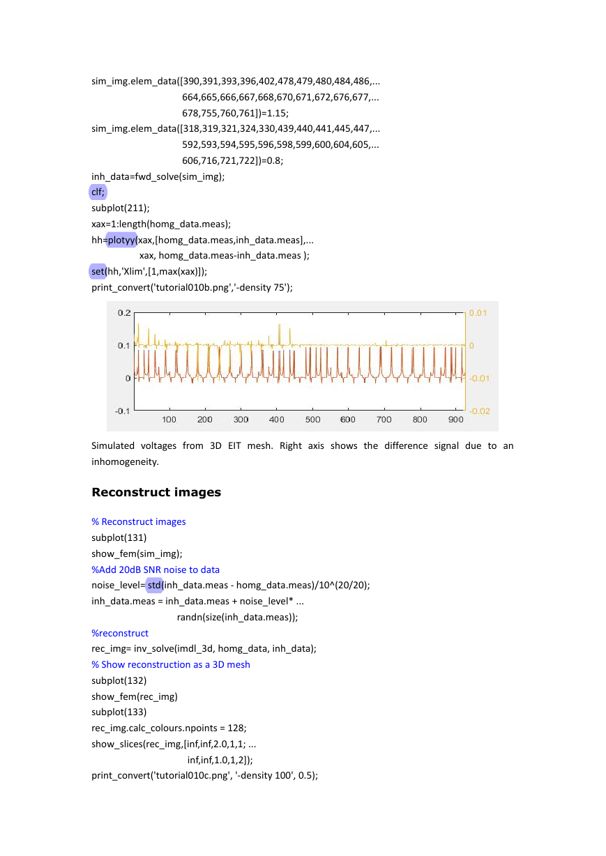
Create a simple 3D fwd_model structure
Reconstruct images
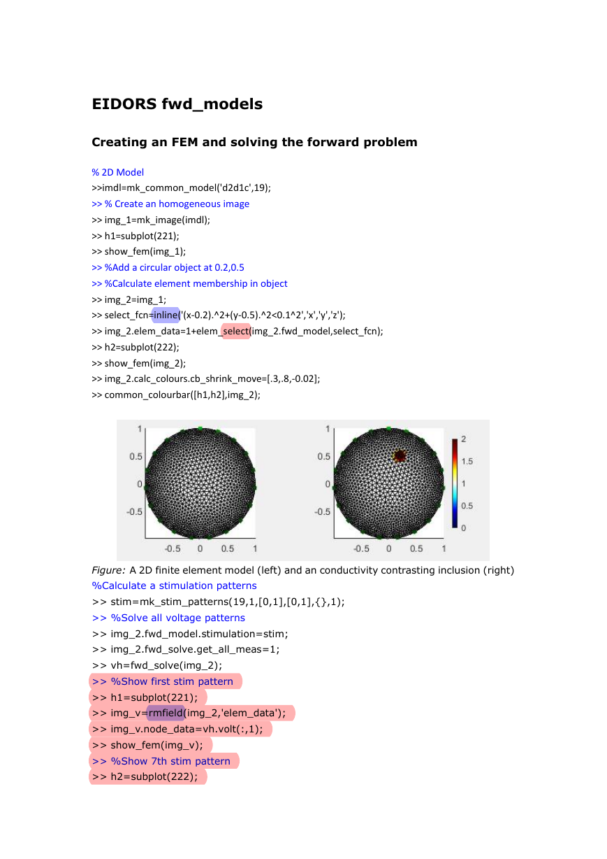
EIDORS fwd_models
Creating an FEM and solving the forward problem
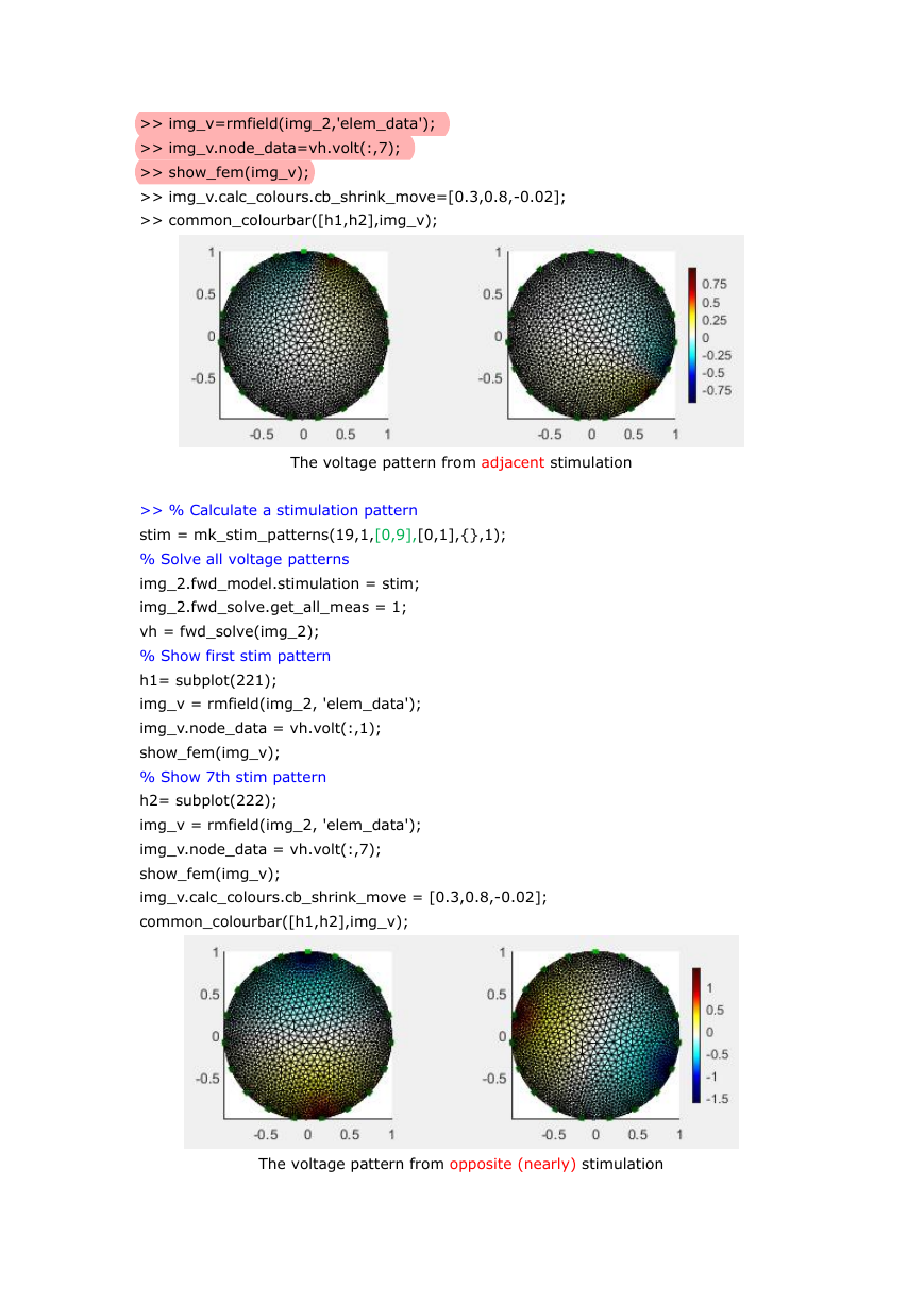
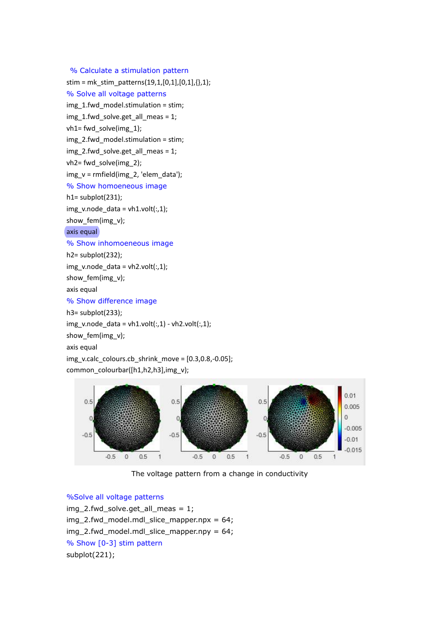
Voltage and Current stimulation
Current (Dirichlet) boundary conditions
Voltage (Neumann) and Current (Dirichlet) boundary
EIDORS fwd_models
Creating an FEM and solving a 3D forward problem
Viewing surface and depth voltages
Create a simple 3D model (electrodes at 170° and 1
Show voltage on surface
Show vertical slices (internal)
Adding contrasts to adjust surface voltages
EIDORS image reconstructions
EIDORS data structures: the inv_model
Reconstruction of real and complex components
Simulation of data with real and complex component
Reconstruction of real and complex changes
Reconstruction of real and complex changes (tank m
EIDORS image reconstructions
Construcxtion of a simple 3D model and image recon
Simulate Voltages
Reconstruction
Gauss Newton solvers in 3D
Simulation Model
Reconstruction with GN solver
Reconstruction with GN solver with hyperparameter
Reconstruction with constrained GN solver
Absolute and Difference solvers
Get data from the RPI tank phantom
Build a good FEM of the phantom
Load and preprocess data
Difference imaging
Estimating actual conductivities
Absolute solvers as a function of iteration
Sensitivity of EIT and Reconstruction
Sensitivity of EIT in 2D
Reconstruction from each component
Compare 2D image reconstructions
Compare 3D image reconstructions
Algorithm Performance
GREIT Test Parameters for different algorithms
Simulate 3D object
Simulate target positions
Gauss-Newton Reconstruction Matrix
Calculate and show GREIT parameters
GN reconstruction vs Backprojection
Calculate the nodal voltage field
Calculate Equipotential lines
Create 2D Model and simulate measurements
Image reconstruction with GN (NOSER) and Backproje
GN vs Sheffield Backprojection
Contrasts in EIT
Overview of EIT contrast signal
Creating an FEM and solving the forward problem
Create table with effect of elliptical shape and c
The effect of contact impedance
Simulation Model
Current Near Top Electrode
Current Stream Lines
EIDORS fwd_models
Solving the forward problem for EIT in 2D with hig
Iterate over model options (including solver and J
EIDORS fwd_models
Solving the forward problem for EIT in 3D with hig
Iterate over model options (including solver and J
EIDORS fwd_models
Complete electrode model (CEM) convergence study u
Methods and Results
Solving onto Nodes vs Elements
Solving onto Nodes vs Elements
Reconstructing onto elements
Reconstructing onto nodes
Iterative Gauss Newton reconstruction in 3D
Reconstruction with different iterations
Residuals 残差
Iterative Gauss Newton reconstruction in 3D
GN reconstruction
TV reconstruction vs iteration
Compare selection of hyperparameters for Total Var
Simluation object
Create TV reconstruction model
Reconstruction with no noise
Reconstruction with 20db SNR noise
Image reconstruction of moving objects
Sample Data
Reconstruction Algorithms
Image Reconstruction
Image Reconstruction Movies
Reconstructing with electrode errors
Eliminating Electrodes
Detecting and automatically eliminating electrodes
Simulation of voltages over time due to transient
Absolute Imaging: Non-Linear Gauss Newton Image R
Cheating with EIDORS
Sample Problem: The happy transform
Approach #1: Careful selection of noise
Approach #2: Careful selection of priors
Approach #3: Edge based priors
Introduction to dual models
Simulated data
Simple Example: Dual model using multi-element par
Image Reconstructions
Example #2: Fine and Coarse meshes
Dual Models − Coarse model partially covers fine m
Coarse and Fine models
Simulated data
Reconstruction models
Reconstructed images (projected to fine mesh)
Reconstructed images (projected to coarse mesh)
Two and a half dim (2½D) image reconstruction
Fourier Approximation
2D + 3D = 2.5D
Model of a 2½D cross-section of a pipe
Simulate an elliptical fluid moves in the pipe
Create reconstruction model
Dual Models to reconstruct a slice of a volume
Create reconstruction model
Image reconstructions
Simpler reconstruction model
Image reconstructions
Dual Models using a rectangular mesh of a volume
Rectangular mesh represented as a triangular FEM
Dual mesh correspondance
Simulation Data
Reconstruct Images
3D-3D Dual Models
Electrode movement reconstruction for simulated 2
Electrode movement reconstruction for simulated 3D
Strange Effect: Opposite vs Adjacent measurement/
Strange Effect: Conformal deformations of boundar
Create a simple model and deform it
Solve the fwd problem on the flat and deformed mod
Unexpected Effect: Imaging with absolute value of
Stimulation Patterns
Simulation Image
Reconstruct without/with Absolute Value
Strategy #1 for absolute values
Strategy #2 for absolute values
Anisotroic deformations of medium shape
Create a simple resistor model and calculate curre
Deform the model and recalculate streamlines
Create isotropic conductivity patterns and recalul
Banana-shaped minima region in objective function
Basic EIDORS data structures
Basic EIDORS data structures: the fwd_model
Modifying EIDORS data structures and models
EIDORS Stimulation patterns
Using 16 electrodes from a 32 electrode model
Reconstruct images with different electrode placem
EIDORS data structures and Variables
What version am I running?
Controlling Output Images
Image Output Resolution
Image Reference Colours
Colour Mapping in the image
EIDORS display functions and control of colours
Colour Mapping in the image
Create a demo image
Change colour mapping parameters: greylev
Change colour mapping parameters: clim
Change colour mapping parameters: sat_adj
Change colour mapping parameters: window_range
Colours and lung images
Customizing EIDORS
Colours
Cache
Default functions
Images of the Pont Péan region
Create 3D FEM model of the terrain
Create 2½D inverse model
Reconstruct the data
Using EIDORS to image geophysics
Borehole model
Create 3D FEM model of the gallery and load homoge
Create forward model. Calculate the difference (re
Reconstruct image and show residual.
Show reconstructed images
Simulating Geophysical measurements around a bore
Create 3D FEM model of the gallery
Place a simulated contrast
Reconstruct images (using full 3D reconstruction)
Reconstruct images (on a 2D simple slice)
Reconstruct images (on a 2D conforming geometry)
Simulation of 3D surface electrode patterns.
Simulate 3D data
Create 3D forward model and reconstruction model
Inversion (using a difference solver)
Create geophysical stimulation patterns and draw
Create 3D FEM model for a horizontal profile
Create a stimulation pattern with a Wenner protoco
Create a stimulation pattern with a Schlumberger p
Create a stimulation pattern with a Dipole-dipole
Case of borehole measurements (or any vertical acq
Case of circumferential measurements around a circ
Case of circumferential measurements around a cavi
Case of circumferential measurements around a cyli
FEM Models Prepackaged with EIDORS
2D FEM Models
Model Reduction
Build Models
Reduce Model
Find Appropriate Resistors
Using Netgen to create cylindrical EIDORS Models
Simple 3D cylinder. Radius = 1. No electrodes
Simple 2D cylinder. Radius = 2. Set minsize to ref
3D cylinder. Radius = 1. 2 planes of 8 elecs with
3D cylinder. Radius = 1. 6 circ elecs with elec re
3D cylinder. Radius = 1. 7 rect elecs with no refi
2D cylinder. Radius = 1. 11 rect elecs with refine
2D cylinder. Radius = 1.5. Refined(0.1). 11 elecs
2D cylinder. elecs at 0, 90 and 120 degrees
2D cylinder. elecs at 0 (large,refined) and 90 (sm
% 3D cylinder. elecs at 0, 30, 60, 90 in planes
3D cylinder. Various elecs at 0, 30, 60, 90 in pla
Simple 3D cylinder with a ball
3D cylinder with 8 electrodes and cube
3D cylinder with inner cylinder
2D cylinder with 8 electrodes and hole
2D cylinder with 9 electrodes and inner cylinder
2D cylinder with 16 electrodes and inner cylinder
3D cylinder with two rows of electrodes and ellips
Using Netgen to create elliptical EIDORS Models
Simple 3D ellipse. Major, minor axes = [1.5, 0.8].
Simple 2D cylinder. Axes = [1.5,0.8]. Refined to 0
3D cylinder. Axes = [1.5,0.8]. 2 planes of 8 elecs
3D cylinder. Axes= [1.3,1] = 1. 7 rect elecs with
2D cylinder. Axes = [1.2,0.8]. 11 rect elecs with
2D cylinder. elecs at 0, 90 and 120 degrees
3D cylinder. Various elecs at 0, 30, 60, 90 in pla
Simple 3D cylinder with a ball
3D cylinder with a two separate balls
Using new ng_mk_geometric_models interface
1: Simple 3D cylinder. Radius = 1 with no electrod
2: Simple 3D cylinder. Radius = 1 with 16 spherica
3: Simple 3D cylinder. Radius = 1 with 16 cylindri
4: 3D Cylinder with electrodes which stick out of
5: 3D Cylinder with electrodes which stick out of
6: 3D Cylinder with electrodes which stick out of
7: 3D Cylinder and sphere with electrodes
8: 3D Cylinder and sphere with electrodes
9: 3D Cylinder with inner cylinder
10: 3D Cylinder and sphere with inner objects
11: 3D Cylinder and sphere with inner objects
12: 3D Cone with electrodes
13: 3D Cone with electrodes
14: 3D Cones and cylinders with electrodes
15: 3D Cube
16: 3D Cube with holes
18: 3D Cube with max_edge_length
19: 3D Parallelepiped
20: 3D Wedge(楔子)
21: ellipsoid
22: ellipsoid
23: cropped cylinder
24: cropped cylinder
25: cylinder with hole
26: cone with hole
27: torus(环面)
28: torus
29: Cylinder with electrodes
30: Cylinder with ball
31: Cylinder with many ball
32: Cylinder with point electrodes
33: Cylinder with point and round electrodes
34: Extrusion
35: Extrusion
36: Extruded torus
37: Lots of electrodes
38: Inclusion in an object
Using Netgen to create extruded EIDORS Models
Extruded 3D shape with 9 rectuangular electrodes
Extruded 3D shape with mesh refinement and 5 large
Extruded 3D shape mesh with boundary interpolation
2D shape mesh boundary interpolation
2D shape with object and specific electrode positi
3D shape with two objects and no electrodes
3D shape with custom electrodes
View of an electric fish in a tank
Model a 3D tank with 8 electrodes and an elliptica
Create stim_patterns and meas_patterns for the fis
Solve for the voltage distribution in the tank
Solve for the voltage distribution near the fish's
Using Netgen to create general (arbitrary) EIDORS
Shape 1
Shape 2
Shape 3
Shape 4
Shape 5
Shape 6
Shape 7
Shape 8
Shape 9
Shape 10
Shape 11
Shape 12
Shape 13
Shape 14
Shape 15
Shape 16
Shape 17
Shape 18
Internal electrodes
Electrode in a hole in the model
Specifying the electrode boundary to EIDORS
Using Netgen to simulate fwd and inverse solutions
Model a 2D tank with 8 electrodes
Simulate a 2D tank with 8 electrodes with adjacent
Simulate a 2D tank with 8 electrodes with differen
Simulate a voltages for a change in conductivity
Voltage patterns for a change in conductivity
Simple image reconstruction
Effects of the Meshsize parameter in Netgen
Setup: use default meshsize
Simulate a moving 2D target on a fixed mesh
Simulate a moving 2D target on a fixed mesh
Step 2: Simulate movement
2D Geophysical models using square mesh elements
Internal Electrodes
Splitting and joining models
Cropping models (2D)
Viewing EIDORS images with Mayavi
Install Mayavi
Calculate image and save to a vtk file
GREIT Reconstruction Examples
Simulate 3D object
Calculate GREIT Reconstruction Matrix
Reconstruction Model (Circular model)
GREIT Reconstruction in 3D
Model of a tank with an object moving vertically
GREIT 2D
GREIT 3D
GREIT 3D − 2D slices
3D GREIT Reconstruction
GREIT Reconstruction For different Model Geometri
Simulation model
Calculate GREIT reconstruction matrices for variou
GREIT Reconstruction for multiple electrode layers
Simulation model
GREIT Test Parameters
Comment
Algorithm Performance
GREIT Test Parameters for different algorithms
Simulate 3D object
GREIT Reconstruction Matrix
Simulation model


 2023年江西萍乡中考道德与法治真题及答案.doc
 2012年重庆南川中考生物真题及答案.doc
 2013年江西师范大学地理学综合及文艺理论基础考研真题.doc
 2020年四川甘孜小升初语文真题及答案I卷.doc
 2020年注册岩土工程师专业基础考试真题及答案.doc
 2023-2024学年福建省厦门市九年级上学期数学月考试题及答案.doc
 2021-2022学年辽宁省沈阳市大东区九年级上学期语文期末试题及答案.doc
 2022-2023学年北京东城区初三第一学期物理期末试卷及答案.doc
 2018上半年江西教师资格初中地理学科知识与教学能力真题及答案.doc
 2012年河北国家公务员申论考试真题及答案-省级.doc
 2020-2021学年江苏省扬州市江都区邵樊片九年级上学期数学第一次质量检测试题及答案.doc
 2022下半年黑龙江教师资格证中学综合素质真题及答案.doc