Journal of Mathematical Finance, 2020, 10, 242-254
https://www.scirp.org/journal/jmf
ISSN Online: 2162-2442
ISSN Print: 2162-2434
Analyzing China’s Term Structure of Interest
Rates Using VAR and Nelson-Siegel Model
Minjie Ding
Peking University, Beijing, China
How to cite this paper: Ding, M.J. (2020)
Analyzing China’s Term Structure of In-
terest Rates Using VAR and Nelson-Siegel
Model. Journal of Mathematical Finance,
10, 242-254.
https://doi.org/10.4236/jmf.2020.102015
Received: January 20, 2020
Accepted: May 8, 2020
Published: May 11, 2020
Copyright © 2020 by author(s) and
Scientific Research Publishing Inc.
This work is licensed under the Creative
Commons Attribution International
License (CC BY 4.0).
http://creativecommons.org/licenses/by/4.0/
Open Access
Abstract
China’s bonds market has developed rapidly in recent years. A further study
of interest rate term structure is essential. Nelson-Siegel model is widely used
to fit interest rate term structure around the world. In this essay, we try to
find out whether Nelson-Siegel model is efficiency in China, and which mod-
el is most efficient among some typical variants of Nelson-Siegel model. After
brief theoretical introduction, we conduct empirical analysis, which contains
two sections. In the first session, we focus on fitting Chinese interest rate
term structure using Nelson-Siegel model, and fitting efficiency turns out to
be pretty good. In the second section, we establish a VAR model with ma-
croeconomic variables to predict parameters in Nelson-Siegel model, and use
the combination of VAR and NS model to predict interest rate term structure
in 2019 and 2020 respectively. Also, in terms of prediction efficiency, VAR
(Macro)-NS model performs better than both VAR-NS model without ma-
croeconomic variables and simple NS model.
Keywords
China’s Term Structure, Nelson-Siegel Model
1. Introduction
Interest rate is one of most important variables in the financial market, which
can depict the relationship between money supply and money demand. Treasury
bonds are regarded as risk-free interest rate for high credit and low risk. Trea-
sury bond yield curve reflects the relationship between bond yield and term to
maturity, so it is also known as interest rate term structure. Treasury bond yield
curve becomes benchmark for financial products, and it’s critical to financial
market.
China’s treasury bond curve began to form since year 2002. Electronic trea-
DOI: 10.4236/jmf.2020.102015 May 11, 2020
242
Journal of Mathematical Finance
�
M. J. Ding
sury bonds were introduced in 2006, which increased the amount of treasury in-
vestment. By the end of 2019, total market value of China’s bond market reached
97,060 billion RMB, yoy 13.2%, becoming the second largest bond market in the
world.
Scholars and investors all over world have shown great interest in treasury
bond yield curve, for its important role in financial market. Treasury bond yield
curves in different countries present different characters. In China, interest rate
used to be regulated, and it’s not easy to predict interest rate barely from market
prospective. With the progress of interest rate marketization, does China’s trea-
sury bond yield curve becomes more easy to predict? Is the prediction convinc-
ing? This paper will focus on these questions in following discussion.
This paper uses the method put up by Nelson & Siegel (1987), to fit treasury
bond yield curve. This method is practical for few parameters, and each para-
meter has economic meanings. Also, this paper follows the research structure by
Diebold & Li (2006). First, the paper fits China’s treasury bond yield curve using
Nelson-Siegel method and tests its efficiency. After that, the paper establishes
VAR (vector auto-regression model) to predict parameters in Nelson-Siegel
model. Then, the paper gives the predicted treasury bond yield curve of 2020.
Compared with relevant researches conducted by scholars and investor, this
paper does some new work. First, the paper uses yield curve data from CCDC
(China Central Depository & Clearing Co., Ltd.,
http://www.ccdc.com.cn/ccdc/en/index.shtml) as raw data, while other re-
searchers usually use specific traded treasury bond in market. CCDC has already
filtered market noise when CCDC calculates yield rate. Also, regulatory depart-
ment has assigned CCDC’s treasury bond yield curve as pricing benchmark. For
example, China Banking Regulatory Commission requires commercial banks to
use CCDC’s treasury bond yield rate as benchmark of risk management. Second,
based on trade experience in Chinese bond market, the paper introduced several
typical macroeconomic variables into dynamic Nelson-Siegel model, and estab-
lished VAR(Macro)-NS model. Third, in order to test the efficiency of
VAR(Macro)-NS model, this paper introduces a VAR-NS model and a NS mod-
el. In addition, although there are already scholars around the world discussing
the effect from macro variables on term structure, the importance of this topic is
not highlighted in China, partly because of long-term regulated interest rate
market and difficulty to get raw market data. This paper is first to fully exam ef-
fect from macro variables on term structure using most proper market data in
China market.
The remainder of this paper is as follows. Section 2 shows literature review of
Nelson-Siegel model, including recent research done by Chinese scholars. Sec-
tion 3 gives brief introduction to Nelson-Siegel model. Section 4 describes how
we estimate the level, slope and curvature factors of the yield curve, and we test
whether Nelson-Siegel model can fit Chinese treasury bond yield curve well.
Section 5 examines predictive ability and gives our predicted yield curve based
243
Journal of Mathematical Finance
DOI: 10.4236/jmf.2020.102015
�
M. J. Ding
DOI: 10.4236/jmf.2020.102015
on VAR(Macro)-NS model.
2. Literature Review
As scholars and investors use yield term structure more frequently, more relative
models come up.
Nelson-Siegel model was first proposed by Nelson and Siegel (1987). This
model is widely favored, for its intuitive economic explanation, less parameters
to estimate and good fitting performance. However, Nelson-Siegel model fails to
produce a multi-peak yield curve. Svensson (1994) added an exponential poly-
nomial to solve the problem, and got Nelson-Siegel-Svensson model. Although
Nelson-Siegel-Svensson model can generate a multi-peak yield curve, too many
parameters makes it too sensitive to initial value.
Nelson-Siegel models are widely used both by academic research and gov-
ernment policy. According to report from BIS (2005) [1], central banks of Bel-
gium, Finland, France, Italy and Span use Nelson-Siegel models to estimate yield
term structure, and centrals banks of US, Canada, UK, German and Switzerland
choose Nelson-Siegel-Svensson model.
Dynamic Nelson-Siegel model was first set up by Diebold and Li (2006) [2].
They assumed that factors of NS model follow AR (1) process. Christensen, Di-
ebold and Rudebusch (2009) [3] consider no-arbitrage restriction in DNS model,
which is called AFDNS model. Koopman, Malle and Van (2010) [4] add
GARCH process into DNS model.
In China, Shen (2010) [5] applied DNS model to Chinese inter-bank market.
Wang (2010) studied no-arbitrage DNS model and found the slope factor has
closer correlation with macroeconomics variables. Shen and Shuai (2017) [6]
decreased parameter numbers in Lengwiler and Lenz’s (2010) [7] model, they
introduced VARMA (1, 1) into DNS model and ensure the independence of
impulse from factors.
In addition, many scholars and investors began to explore the relationship
between interest rate and macroeconomic variables.
Ang and Piazzesi (2003) [8] added macroeconomic variables to interest rate
model. They got a better predictability, and found that 85% of yield volatility
could be explained by macroeconomic variables. Based on this work, Bikbov and
Chernov (2010) [9] proposed a model without restrictions on the number of la-
tent variables. Also, discussion about forecast horizons came up, Hordahl (2006)
and Moench (2008) [10] found model with macro variables had better forecast-
ing performance only for longer prediction horizons, while de Pooter (2010) and
Altavilla (2014) outperformed random walk benchmarks only for short-term
maturities at shorter horizons. Coroneo (2016) [11] added backward-looking
macroeconomic variables into term structure model, and his model performed
better than random walk forecasts from 3 to 24 months ahead. It is argued that
macro variables is useful particularly in certain years, such as in recessionary pe-
riods. This argument is supported by evidence provided by Guidolin and Pedio’s
244
Journal of Mathematical Finance
�
M. J. Ding
(2019) [12], whose models with monetary policy variables significantly increased
predictive ability during 2008 financial crisis.
Interest rate in China was partially regulated until recent years. As a result,
Chinese scholar didn’t pay much attention to macroeconomic variables and
yield term structure before 2010. In recent years, relevant studies came up, as
interest rate realized liberalization. Zeng and Niu (2013) became first Chinese
scholar who got term structure of real interest rate and inflation rate, using
no-arbitrage models. They also found that inflation rate affected more on
short-term yields, while real interest rate affected more on long-term yields.
Qiang and Hou (2018) [13] built an affine interest rate model based on bench-
mark interest rate, market liquidity and risk premium, which explained the term
structure well. They found that benchmark interest rate is determinant to other
term yields, and market liquidity influence more on short-term yields, while risk
premium affects more on long-term yields.
3. Brief Introduction to Nelson-Siegel Model
In 1987, Nelson and Siegel first use Nelson-Siegel model to fit yield curve, and
the model is as follows.
y
( )
τ β β
2
=
+
1
∗
−
λτ
1 e
−
λτ
+
β
3
∗
−
λτ
1 e
−
λτ
−
λτ
−
e
(1)
Diebold and Li said that yield rate should change with time, and put forward
Dynamic Nelson-Siegel model, and the model is as follows.
y
t
( )
τ β β
2
=
+
t
1
∗
t
λτ
−
1 e
−
λτ
+
β
t
3
∗
λτ
−
1 e
−
λτ
λτ
−
−
e
(2)
In the formula above, t represents a specific time point. τ represents time to
ty τ represents the yield rate of a treasury bond with τ to matur-
( )
β β β and λ are parameters to be estimate.
maturity.
ity at time t.
• As τ approaches infinity, we get
( )
τ β
t
1
y
lim t
→∞
τ
1tβ is regarded as
1tβ will change the overall yield rate of a
. So
=
t
1
,
,
2
horizontal parameter. Change of
treasury bond.
t
3
t
• As τ approaches zero, we get
y
−
t
( )
0
( )
0
β
t
1
β
2
y
t
y
t
−
=
=
t
get
ter.
( )
y
lim t
τ β β
2
0
τ
→
(
)
∞ . So
=
. After transposition, we
2tβ is regarded as slope parame-
+
t
1
t
• When τ is a normal number around 60, which means the treasury bond
+
−
=
y
t
β
t
1
( )
0
0.5
y
t
)
60
(
=
has 5 years (60 months) to maturity, we approximately get
(
y
∗
β
t
t
2
)
( )
β
−
τ
t
3
vature parameter.
The right side of formula divides the yield rate into three parts. The first item
1tβ , which affects long-term yield rate. We can call it long-term factor. The
β
. After transposition, we get
t
3
(
y
−
t
3tβ is usually regarded as cur-
0.5
+
∗
(
( )
y
τ
t
)
∞ . So
)
is
second item is
DOI: 10.4236/jmf.2020.102015
1 e λτ
−−
λτ
, when τ approaches infinity, this item approaches ze-
245
Journal of Mathematical Finance
�
M. J. Ding
DOI: 10.4236/jmf.2020.102015
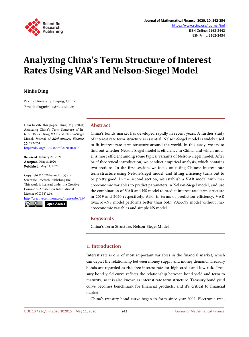
ro, which means this item affect yield rate more in short term, as shown in Fig-
ure 1. We can call it short-term factor. The third item is
λτ
−
1 e
−
λτ
λτ
−
−
e
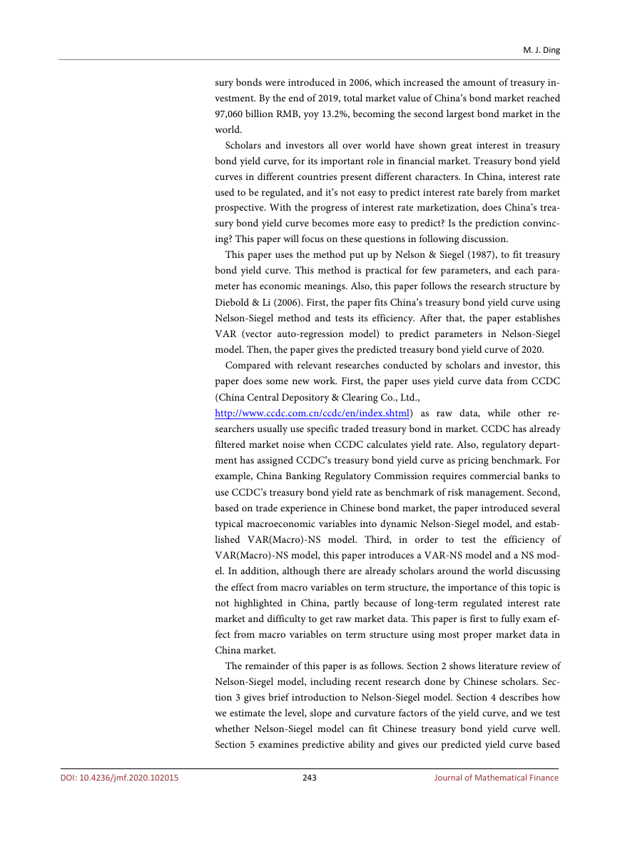
, as
τ approaches infinity or zero, the third item approaches zero, which means its
effect is around medium-term, as shown in Figure 2, so we can call it me-
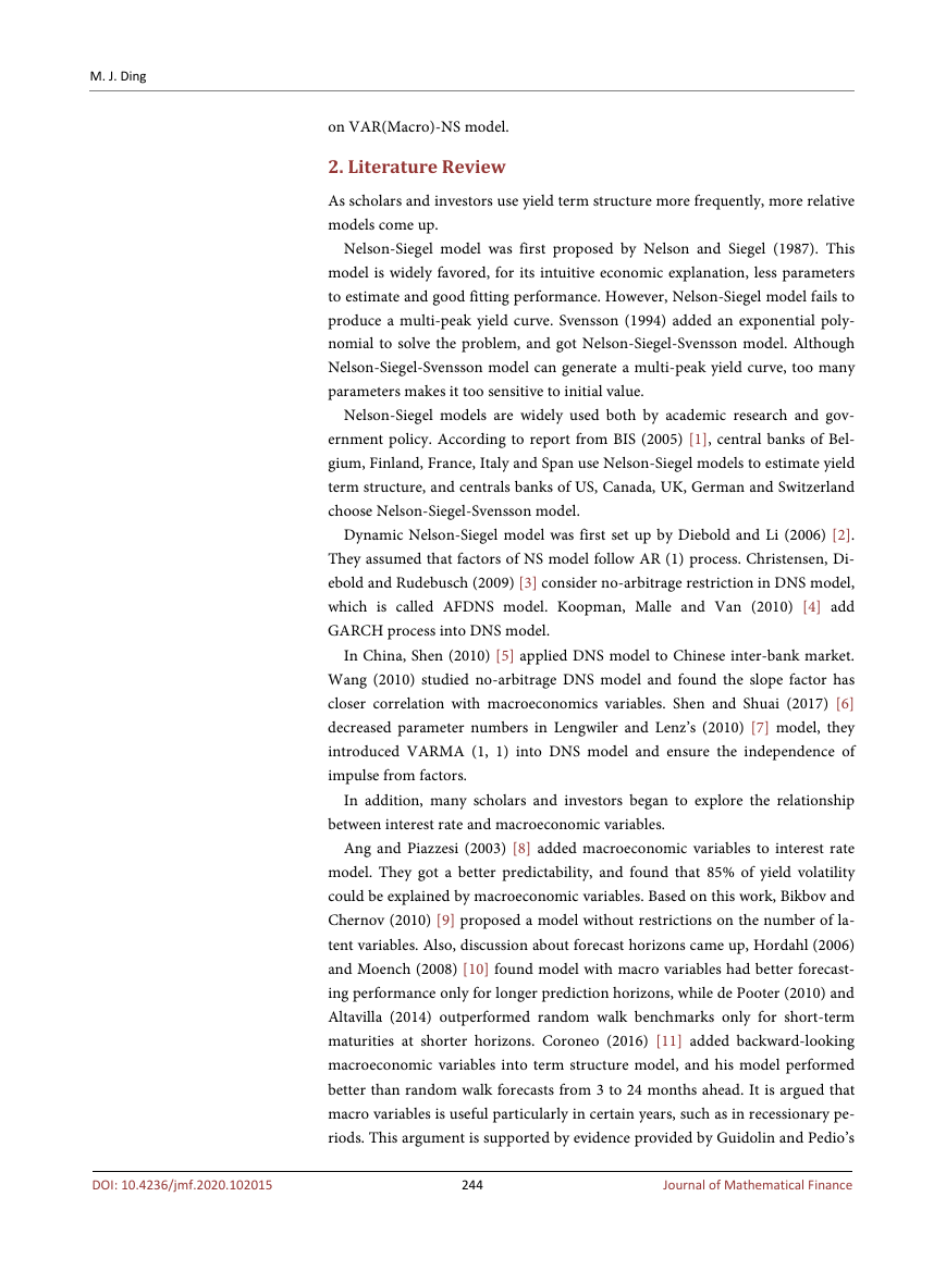
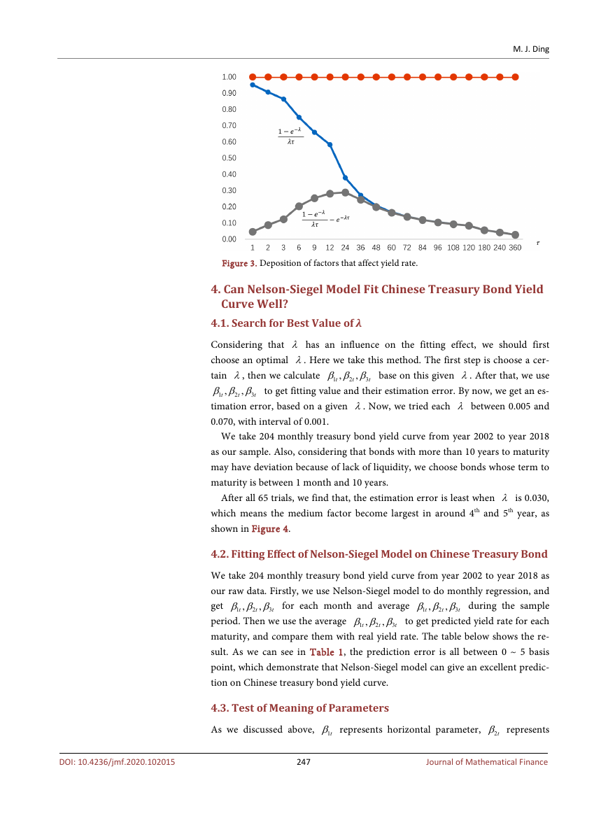
dium-term factor. So all factors that affect yield curve can be divided into these
three group, as shown in Figure 3.
λ is usually given previous to other work. On the one side, λ determines
when
λτ
−
1 e
−
λτ
λτ
−
−
e
will reach largest value. On the other side, λ determines
the speed
1 e λτ
−−
λτ
decreases with time. Diebold and Li (2006) take
λ=
0.0609
,
which means medium factor reaches largest in 30th month.
Figure 1. 1 e λτ
−−
λτ
trend (assuming
0.1λ=
).
Figure 2. 1 e
−
λτ
−
λτ
−
λτ
−
e
trend (assuming
0.1λ=
).
246
Journal of Mathematical Finance
�
M. J. Ding
Figure 3. Deposition of factors that affect yield rate.
4. Can Nelson-Siegel Model Fit Chinese Treasury Bond Yield
Curve Well?
4.1. Search for Best Value of λ
Considering that λ has an influence on the fitting effect, we should first
choose an optimal λ. Here we take this method. The first step is choose a cer-
tain λ, then we calculate
β β β base on this given λ. After that, we use
t
1
β β β to get fitting value and their estimation error. By now, we get an es-
t
1
timation error, based on a given λ. Now, we tried each λ between 0.005 and
0.070, with interval of 0.001.
,
,
,
,
2
3
2
3
t
t
t
t
We take 204 monthly treasury bond yield curve from year 2002 to year 2018
as our sample. Also, considering that bonds with more than 10 years to maturity
may have deviation because of lack of liquidity, we choose bonds whose term to
maturity is between 1 month and 10 years.
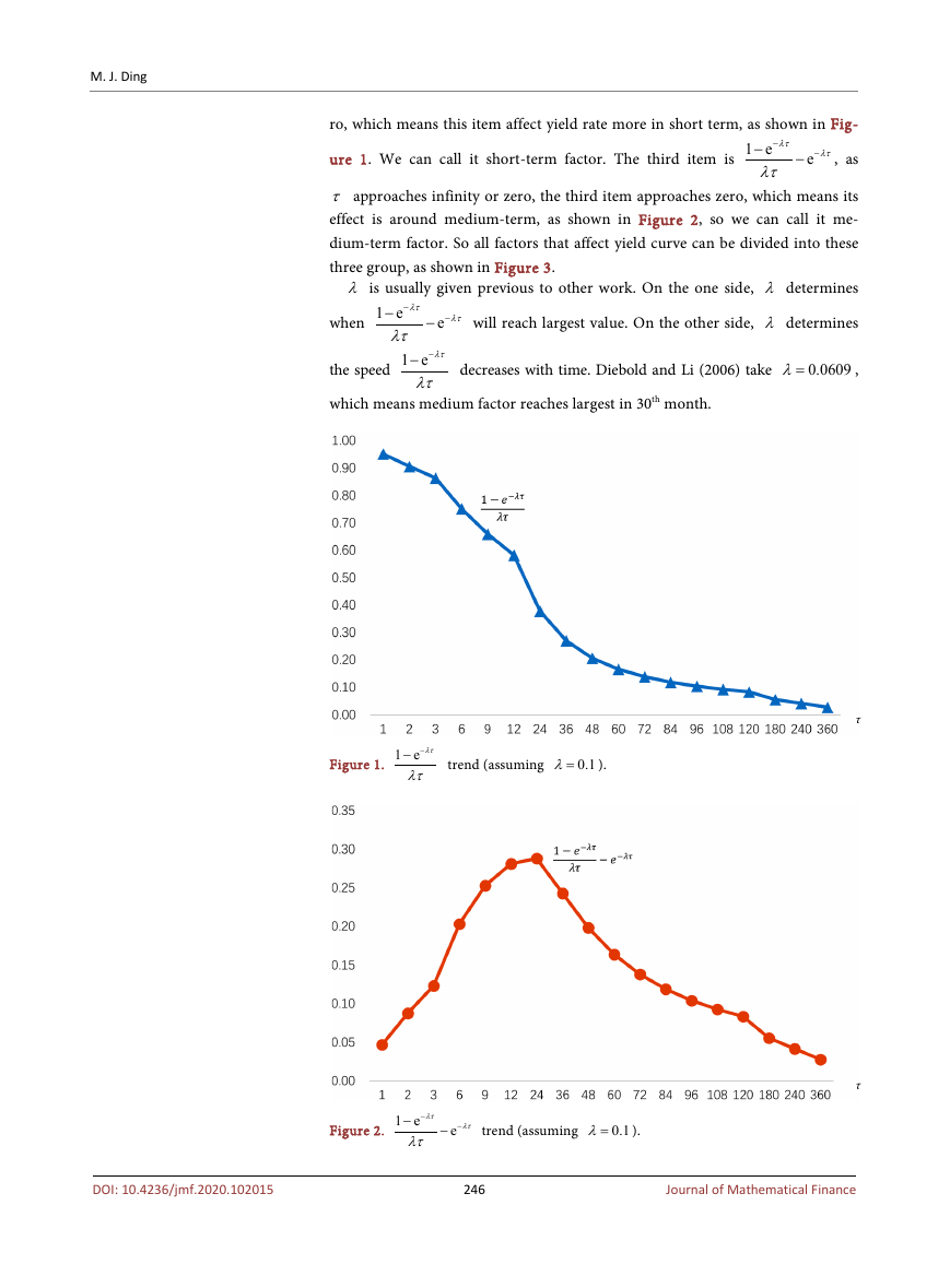
After all 65 trials, we find that, the estimation error is least when λ is 0.030,
which means the medium factor become largest in around 4th and 5th year, as
shown in Figure 4.
t
t
2
,
,
β β β for each month and average
t
1
4.2. Fitting Effect of Nelson-Siegel Model on Chinese Treasury Bond
We take 204 monthly treasury bond yield curve from year 2002 to year 2018 as
our raw data. Firstly, we use Nelson-Siegel model to do monthly regression, and
get
β β β during the sample
t
1
period. Then we use the average
β β β to get predicted yield rate for each
t
1
maturity, and compare them with real yield rate. The table below shows the re-
sult. As we can see in Table 1, the prediction error is all between 0 ~ 5 basis
point, which demonstrate that Nelson-Siegel model can give an excellent predic-
tion on Chinese treasury bond yield curve.
,
,
,
,
2
3
3
2
t
t
t
3
t
4.3. Test of Meaning of Parameters
As we discussed above,
1tβ represents horizontal parameter,
2tβ represents
247
Journal of Mathematical Finance
DOI: 10.4236/jmf.2020.102015
�
M. J. Ding
slope parameter and
3tβ represents curvature parameter in Nelson-Siegel
model. While in real trading market, we can use yield rate of bonds with 10 year
to maturity to represent horizontal level of yield curve. Also, real slope is often
approximately calculated by substracting 1-year yield rate from 10-year yield
rate. Moreover, we can use “(10-year yield rate - 10-year yield rate) - (5-year
yield rate - 1-year yield rate)” to approximately represent real curvature. Our
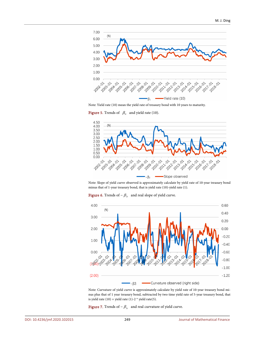
calculation result is in Table 2. We find that the correlation between
1tβ and
real horizontal level is 0.866, the correlation between
2tβ and real slope is
−0.964 and the correlation between
3tβ and real curvature −0.554. These three
parameters all have close relationship with real observed values. Figure 5, Fig-
ure 6 and Figure 7 show the trends of three relationships mentioned above,
which further manifest the close correlation.
Table 1. Real yield rate vs. fitted yield rate in 2002-2018.
Figure 4. Average absolute fitting error from Nelson-Siegel model with different λ.
2
3
6
9
12
24
36
48
60
72
84
96
108
120
2.3806 2.4132 2.4810 2.5256 2.5745 2.7624 2.9253 3.0673 3.1769 3.3090 3.3960 3.4719 3.5313 3.5837
2.3767 2.3952 2.4498 2.5030 2.5547 2.7470 2.9166 3.0650 3.1941 3.3063 3.4037 3.4882 3.5617 3.6258
−0.38 −1.80 −3.12 −2.26 −1.98 −1.54 −0.87 −0.23
4.21
−0.27
1.73
0.77
1.63
3.05
Time to maturity τ (month)
Average historical yield rate
(%)
Fitted yield rate (%)
Predicted error (BP)
DOI: 10.4236/jmf.2020.102015
Table 2. Correlation between estimated parameters and real term structure.
Observed height
of yield curve
Observed slope
of yield curve
Observed curvature of yield curve
Yield rate (10)
Yield rate (10) minus
yield rate (1)
Yield rate (10) plus yield rate (1), minus
two times yield rate (5)
0.866
−0.074
0.341
0.398
−0.964
0.031
−0.010
0.147
−0.554
1tβ
2tβ
3tβ
Note: Yield rate (x) means the yield rate of treasury bond with x years to maturity.
248
Journal of Mathematical Finance
�
Note: Yield rate (10) mean the yield rate of treasury bond with 10 years to maturity.
Figure 5. Trends of
1tβ and yield rate (10).
M. J. Ding
Note: Slope of yield curve observed is approximately calculate by yield rate of 10-year treasury bond
minus that of 1-year treasury bond, that is yield rate (10)-yield rate (1).
Figure 6. Trends of − 2tβ and real slope of yield curve.
Note: Curvature of yield curve is approximately calculate by yield rate of 10-year treasury bond mi-
nus plus that of 1 year treasury bond, subtracted by two time yield rate of 5-year treasury bond, that
is yield rate (10) + yield rate (1)-2 * yield rate(5).
Figure 7. Trends of − 3tβ and real curvature of yield curve.
249
Journal of Mathematical Finance
DOI: 10.4236/jmf.2020.102015
�




 2023年江西萍乡中考道德与法治真题及答案.doc
 2012年重庆南川中考生物真题及答案.doc
 2013年江西师范大学地理学综合及文艺理论基础考研真题.doc
 2020年四川甘孜小升初语文真题及答案I卷.doc
 2020年注册岩土工程师专业基础考试真题及答案.doc
 2023-2024学年福建省厦门市九年级上学期数学月考试题及答案.doc
 2021-2022学年辽宁省沈阳市大东区九年级上学期语文期末试题及答案.doc
 2022-2023学年北京东城区初三第一学期物理期末试卷及答案.doc
 2018上半年江西教师资格初中地理学科知识与教学能力真题及答案.doc
 2012年河北国家公务员申论考试真题及答案-省级.doc
 2020-2021学年江苏省扬州市江都区邵樊片九年级上学期数学第一次质量检测试题及答案.doc
 2022下半年黑龙江教师资格证中学综合素质真题及答案.doc