0
2
0
2
r
a
M
1
1
]
G
L
.
s
c
[
1
v
5
2
3
5
0
.
3
0
0
2
:
v
i
X
r
a
Published as a conference paper at ICLR 2020
META-LEARNING CURIOSITY ALGORITHMS
Ferran Alet∗, Martin F. Schneider∗, Tom´as Lozano-P´erez & Leslie Pack Kaelbling
Computer Science and Artificial Intelligence Laboratory
Massachusetts Institute of Technology
Cambridge, MA 02139, USA
{alet,martinfs,tlp,lpk}@mit.edu
ABSTRACT
We hypothesize that curiosity is a mechanism found by evolution that encourages
meaningful exploration early in an agent’s life in order to expose it to experiences
that enable it to obtain high rewards over the course of its lifetime. We formulate
the problem of generating curious behavior as one of meta-learning: an outer
loop will search over a space of curiosity mechanisms that dynamically adapt
the agent’s reward signal, and an inner loop will perform standard reinforcement
learning using the adapted reward signal. However, current meta-RL methods
based on transferring neural network weights have only generalized between very
similar tasks. To broaden the generalization, we instead propose to meta-learn
algorithms: pieces of code similar to those designed by humans in ML papers.
Our rich language of programs combines neural networks with other building
blocks such as buffers, nearest-neighbor modules and custom loss functions.
We demonstrate the effectiveness of the approach empirically, finding two novel
curiosity algorithms that perform on par or better than human-designed published
curiosity algorithms in domains as disparate as grid navigation with image inputs,
acrobot, lunar lander, ant and hopper.
1
INTRODUCTION
When a reinforcement-learning agent is learn-
ing to behave, it is critical that it both explores
its domain and exploits its rewards effectively.
One way to think of this problem is in terms
of curiosity or intrisic motivation: construct-
ing reward signals that augment or even replace
the extrinsic reward from the domain, which in-
duce the RL agent to explore their domain in a
way that results in effective longer-term learn-
ing and behavior (Pathak et al., 2017; Burda
et al., 2018; Oudeyer, 2018). The primary diffi-
culty with this approach is that researchers are
hand-designing these strategies:
it is difficult
for humans to systematically consider the space
of strategies or to tailor strategies for the distri-
bution of environments an agent might be ex-
pected to face.
We take inspiration from the curious behavior
observed in young humans and other animals
and hypothesize that curiosity is a mechanism found by evolution that encourages meaningful ex-
ploration early in an agent’s life. This exploration exposes it to experiences that enable it to learn
to obtain high rewards over the course of its lifetime. We propose to formulate the problem of gen-
erating curious behavior as one of meta-learning: an outer loop, operating at “evolutionary” scale
will search over a space of algorithms for generating curious behavior by dynamically adapting the
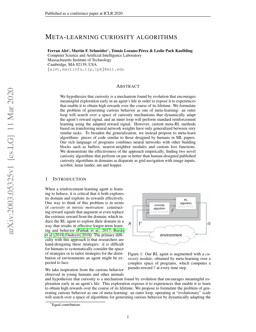
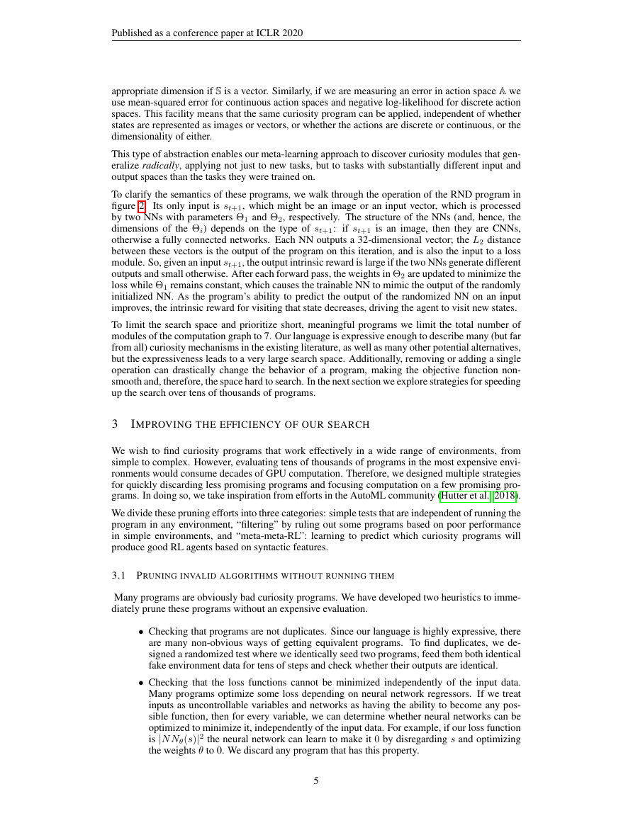
Figure 1: Our RL agent is augmented with a cu-
riosity module, obtained by meta-learning over a
complex space of programs, which computes a
pseudo-rewardr at every time step.
∗Equal contribution.
1
�
Published as a conference paper at ICLR 2020
k≥0 γkrt+k. The outer “evolutionary” search is attempting to find a program
t=0 rt, or another global
agent’s reward signal, and an inner loop will perform standard reinforcement learning using the
adapted reward signal. This process is illustrated in figure 1; note that the aggregate agent, outlined
in gray, has the standard interface of an RL agent. The inner RL algorithm is continually adapting to
its input stream of states and rewards, attempting to learn a policy that optimizes the discounted sum
of proxy rewards
for the curiosity module, so as to optimize the agent’s lifetime returnT
objective like the mean performance on the last few trials.
In this meta-learning setting, our objective is to find a curiosity module that works well given a
distribution of environments from which we can sample at meta-learning time. Meta-RL has been
widely explored recently, in some cases with a focus on reducing the amount of experience needed
by initializing the RL algorithm well (Finn et al., 2017; Clavera et al., 2019) and, in others, for
efficient exploration (Duan et al., 2016; Wang et al., 2017). The environment distributions in these
cases have still been relatively low-diversity, mostly limited to variations of the same task, such
as exploring different mazes or navigating terrains of different slopes. We would like to discover
curiosity mechanisms that can generalize across a much broader distribution of environments, even
those with different state and action spaces: from image-based games, to joint-based robotic control
tasks. To do that, we perform meta-learning in a rich, combinatorial, open-ended space of programs.
This paper makes three novel contributions.
We focus on a regime of meta-reinforcement-learning in which the possible environments the
agent might face are dramatically disparate and in which the agent’s lifetime is very long.
This is a substantially different setting than has been addressed in previous work on meta-RL and it
requires substantially different techniques for representation and search.
We propose to do meta-learning in a rich, combinatorial space of programs rather than
transferring neural network weights. The programs are represented in a domain-specific lan-
guage (DSL) which includes sophisticated building blocks including neural networks complete with
gradient-descent mechanisms, learned objective functions, ensembles, buffers, and other regressors.
This language is rich enough to represent many previously reported hand-designed exploration al-
gorithms. We believe that by performing meta-RL in such a rich space of mechanisms, we will be
able to discover highly general, fundamental curiosity-based exploration methods. This generality
means that a relatively computationally expensive meta-learning process can be amortized over the
lifetimes of many agents in a wide variety of environments.
We make the search over programs feasible with relatively modest amounts of computation.
It is a daunting search problem to find a good solution in a combinatorial space of programs, where
evaluating a single potential solution requires running an RL algorithm for up to millions of time
steps. We address this problem in multiple ways. By including environments of substantially dif-
ferent difficulty and character, we can evaluate candidate programs first on relatively simple and
short-horizon domains: if they don’t perform well in those domains, they are pruned early, which
saves a significant amount of computation time. In addition, we predict the performance of an al-
gorithm from its structure and operations, thus trying the most promising algorithms early in our
search. Finally, we also monitor the learning curve of agents and stop unpromising programs before
they reach all T environment steps.
We demonstrate the effectiveness of the approach empirically, finding curiosity strategies that per-
form on par or better than those in published literature. Interestingly, the top 2 algorithms, to the
best of our knowledge, had not been proposed before, despite making sense in hindsight. We con-
jecture the first one (shown in figure 3) is deceptively simple and that the complexity of the other
one (figure 10 in the appendix) makes it relatively implausible for humans to discover.
2 PROBLEM FORMULATION
2.1 META-LEARNING PROBLEM
Let us assume we have an agent equipped with an RL algorithm (such as DQN or PPO, with all
hyperparameters specified), A, which receives states and rewards from and outputs actions to an en-
vironment E, generating a stream of experienced transitions e(A;E)t = (st, at, rt, st+1). The agent
continually learns a policy π(t) : st → at, which will change in time as described by algorithm A;
2
�
Published as a conference paper at ICLR 2020
may efficiently explore in the outer environment.
so π(t) = A(e1:t−1) and thus at ∼ A(e1:t−1)(st). Although this need not be the case, we can think
i γirt+i, γ < 1 and that, at any
time-step t, always takes the greedy action that maximizes its estimated expected discounted reward.
To add exploration to this policy, we include a curiosity module C that has access to the stream of
state transitions et experienced by the agent and that, at every time-step t, outputs a proxy reward
of A as an algorithm that tries to maximize the discounted reward
rt. We connect this module so that the original RL agent receives these modified rewards, thus
observing e(A,C;E)t = (st, at,rt = C(e1:t−1), st+1), without having access to the original rt.
Now, even though the inner RL algorithm acts in a purely exploitative manner with respect tor, it
Our overall goal is to design a curiosity module C that induces the agent to maximizeT
t=0 rt, for
some number of total time-steps T or some other global goal, like final episode performance. In an
episodic problem, T will span many episodes. More formally, given a single environment E, RL
algorithm A, and curiosity module C, we can see the triplet (environment, curiosity module, agent)
as a dynamical system that induces state transitions for the environment, and learning updates for
the curiosity module and the agent. Our objective is to find C that maximizes the expected original
reward obtained by the composite system in the environment. Note that the expectation is over two
different distributions at different time scales: there is an “outer” expectation over environments E,
and in “inner” expectation over the rewards received by the composite system in that environment,
so our final objective is:
T
t=0
EE
Ert∼e(A,C;E)
rt
.
maxC
2.2 PROGRAMS FOR CURIOSITY
In science and computing, mathematical language has been very successful in describing varied
phenomena and powerful algorithms with short descriptions. As Valiant points out: “the power
[of mathematics and algorithms] comes from the implied generality, that knowledge of one equation
alone will allow one to make accurate predictions about a host of situations not even conceived when
the equation was first written down” (Valiant, 2013). Therefore, in order to obtain curiosity modules
that can generalize over a very broad range of tasks and that are sophisticated enough to provide
exploration guidance over very long horizons, we describe them in terms of general programs in a
domain-specific language. Algorithms in this language will map a history of (st, st+1, at, rt) tuples
into a proxy rewardrt.
Inspired by human-designed systems that compute and use intrinsic rewards, and to simplify the
search, we decompose the curiosity module into two components: the first, I, outputs an intrin-
sic reward value it based on the current experienced transition (st, at, st+1) (and past transitions
(s1:t−1, a1:t−1) indirectly through its memory); the second, χ, takes the current time-step t, the
actual reward rt, and the intrinsic reward it (and, if it chooses to store them, their histories) and
combines them to yield the proxy rewardrt. To ease generalization across different timescales, in
practice, before feeding t into χ we normalize it by the total length of the agent’s lifetime, T .
Both programs consist of a directed acyclic graph (DAG) of modules with polymorphically typed
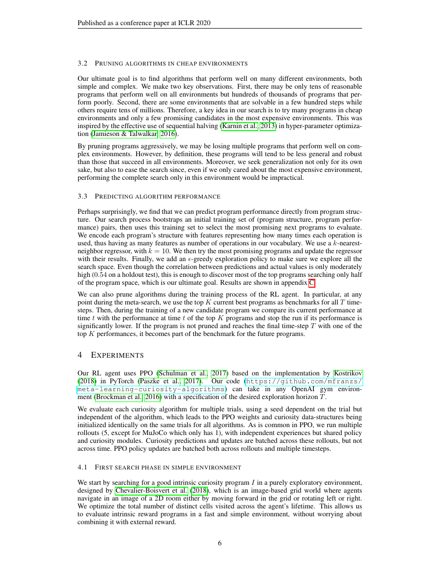
inputs and outputs. As shown in figure 2, there are four classes of modules:
• Input modules (shown in blue), drawn from the set {st, at, st+1} for the I component and
from the set {it, rt} for the χ component. They have no inputs, and their outputs have the
type corresponding to the types of states and actions in whatever domain they are applied
to, or the reals numbers for rewards.
• Buffer and parameter modules (shown in gray) of two kinds: FIFO queues that provide
as output a finite list of the k most recent inputs, and neural network weights initialized at
random at the start of the program and which may (pink border) or may not (black border)
get updated via back-propagation depending on the computation graph.
• Functional modules (shown in white), which compute output values given the inputs from
their parent modules.
3
�
Published as a conference paper at ICLR 2020
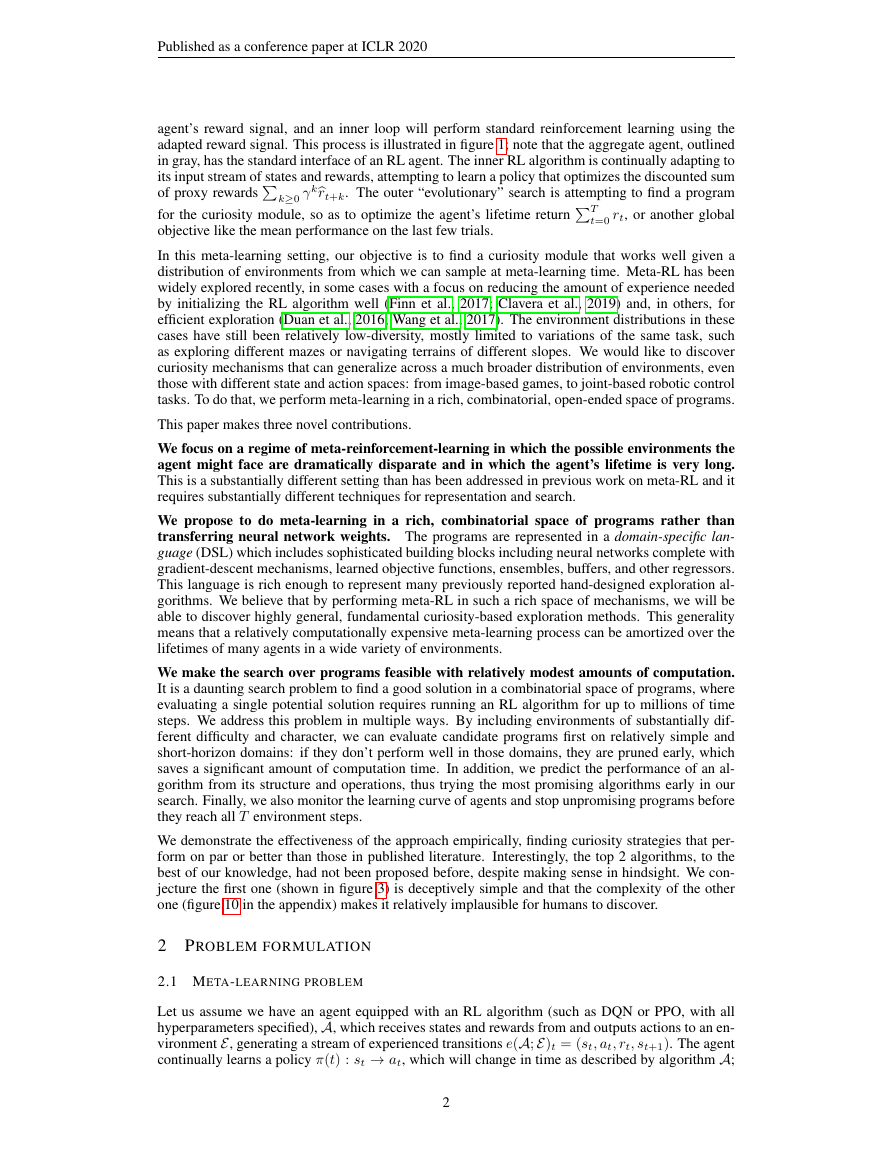
Figure 2: Example diagrams of published algorithms covered by our language (larger figures in the
appendix). The green box represents the output of the intrinsic curiosity function, the pink box is
the loss to be minimized. Pink arcs represent paths and networks along which gradients flow back
from the minimizer to update parameters.
• Update modules (shown in pink), which are functional modules (such as k-Nearest-
Neighbor) that either add variables to buffers or modules which add real-valued outputs
to a global loss that will provide error signals for gradient descent.
A single node in the DAG is designated as the output node (shown in green): the output of this node
is considered to be the output of the entire program, but it need not be a leaf node of the DAG.
On each call to a program (corresponding to one time-step of the system) the current input values
and parameter values are propagated through the functional modules, and the output node’s output
is given to the RL algorithm. Before the call terminates, the FIFO buffers are updated and the
adjustable parameters are updated via gradient descent using the Adam optimizer (Kingma & Ba,
2014). Most operations are differentiable and thus able to propagate gradients backwards. Some
operations are not differentiable, including buffers (to avoid backpropagating through time) and
”Detach” whose purpose is stopping the gradient from flowing back. In practice, we have multiple
copies of the same agent running at the same time, with both a shared policy and shared curiosity
module. Thus, we execute multiple reward predictions on a batch and then update on a batch.
Programs representing several published designs for curiosity modules that perform internal gra-
dient descent, including inverse features (Pathak et al., 2017), random network distillation (RND)
(Burda et al., 2018), and ensemble predictive variance (Pathak et al., 2019), are shown in figure 2
(bigger versions can be found in appendix A.3). We can also represent algorithms similar to novelty
search (Lehman & Stanley, 2008) and EX 2 (Fu et al., 2017), which include buffers and nearest
neighbor regression modules. Details on the data types and module library are given in appendix A.
A crucial, and possibly somewhat counter-intuitive, aspect of these programs is their use of neural
network weight updates via gradient descent as a form of memory. In the parameter update step, all
adjustable parameters are decremented by the gradient of the sum of the outputs of the loss modules,
with respect to the parameters. This type of update allows the program to, for example, learn to make
some types of predictions, online, and use the quality of those predictions in a state to modulate the
proxy reward for visiting that state (as is done, for example, in RND).
Key to our program search are polymorphic data types: the inputs and outputs to each module are
typed, but the instantiation of some types, and thus of some operations, depends on the environment.
We have four types: reals R, state space of the given environment S, action space of the given en-
vironment A and feature space F, used for intermediate computations and always set to R32 in our
current implementation. For example, a neural network module going from S to F will be instanti-
ated as a convolutional neural network if S is an image and as a fully connected neural network of the
4
�
Published as a conference paper at ICLR 2020
appropriate dimension if S is a vector. Similarly, if we are measuring an error in action space A we
use mean-squared error for continuous action spaces and negative log-likelihood for discrete action
spaces. This facility means that the same curiosity program can be applied, independent of whether
states are represented as images or vectors, or whether the actions are discrete or continuous, or the
dimensionality of either.
This type of abstraction enables our meta-learning approach to discover curiosity modules that gen-
eralize radically, applying not just to new tasks, but to tasks with substantially different input and
output spaces than the tasks they were trained on.
To clarify the semantics of these programs, we walk through the operation of the RND program in
figure 2. Its only input is st+1, which might be an image or an input vector, which is processed
by two NNs with parameters Θ1 and Θ2, respectively. The structure of the NNs (and, hence, the
dimensions of the Θi) depends on the type of st+1:
if st+1 is an image, then they are CNNs,
otherwise a fully connected networks. Each NN outputs a 32-dimensional vector; the L2 distance
between these vectors is the output of the program on this iteration, and is also the input to a loss
module. So, given an input st+1, the output intrinsic reward is large if the two NNs generate different
outputs and small otherwise. After each forward pass, the weights in Θ2 are updated to minimize the
loss while Θ1 remains constant, which causes the trainable NN to mimic the output of the randomly
initialized NN. As the program’s ability to predict the output of the randomized NN on an input
improves, the intrinsic reward for visiting that state decreases, driving the agent to visit new states.
To limit the search space and prioritize short, meaningful programs we limit the total number of
modules of the computation graph to 7. Our language is expressive enough to describe many (but far
from all) curiosity mechanisms in the existing literature, as well as many other potential alternatives,
but the expressiveness leads to a very large search space. Additionally, removing or adding a single
operation can drastically change the behavior of a program, making the objective function non-
smooth and, therefore, the space hard to search. In the next section we explore strategies for speeding
up the search over tens of thousands of programs.
3
IMPROVING THE EFFICIENCY OF OUR SEARCH
We wish to find curiosity programs that work effectively in a wide range of environments, from
simple to complex. However, evaluating tens of thousands of programs in the most expensive envi-
ronments would consume decades of GPU computation. Therefore, we designed multiple strategies
for quickly discarding less promising programs and focusing computation on a few promising pro-
grams. In doing so, we take inspiration from efforts in the AutoML community (Hutter et al., 2018).
We divide these pruning efforts into three categories: simple tests that are independent of running the
program in any environment, “filtering” by ruling out some programs based on poor performance
in simple environments, and “meta-meta-RL”: learning to predict which curiosity programs will
produce good RL agents based on syntactic features.
3.1 PRUNING INVALID ALGORITHMS WITHOUT RUNNING THEM
Many programs are obviously bad curiosity programs. We have developed two heuristics to imme-
diately prune these programs without an expensive evaluation.
• Checking that programs are not duplicates. Since our language is highly expressive, there
are many non-obvious ways of getting equivalent programs. To find duplicates, we de-
signed a randomized test where we identically seed two programs, feed them both identical
fake environment data for tens of steps and check whether their outputs are identical.
• Checking that the loss functions cannot be minimized independently of the input data.
Many programs optimize some loss depending on neural network regressors. If we treat
inputs as uncontrollable variables and networks as having the ability to become any pos-
sible function, then for every variable, we can determine whether neural networks can be
optimized to minimize it, independently of the input data. For example, if our loss function
is |N Nθ(s)|2 the neural network can learn to make it 0 by disregarding s and optimizing
the weights θ to 0. We discard any program that has this property.
5
�
Published as a conference paper at ICLR 2020
3.2 PRUNING ALGORITHMS IN CHEAP ENVIRONMENTS
Our ultimate goal is to find algorithms that perform well on many different environments, both
simple and complex. We make two key observations. First, there may be only tens of reasonable
programs that perform well on all environments but hundreds of thousands of programs that per-
form poorly. Second, there are some environments that are solvable in a few hundred steps while
others require tens of millions. Therefore, a key idea in our search is to try many programs in cheap
environments and only a few promising candidates in the most expensive environments. This was
inspired by the effective use of sequential halving (Karnin et al., 2013) in hyper-parameter optimiza-
tion (Jamieson & Talwalkar, 2016).
By pruning programs aggressively, we may be losing multiple programs that perform well on com-
plex environments. However, by definition, these programs will tend to be less general and robust
than those that succeed in all environments. Moreover, we seek generalization not only for its own
sake, but also to ease the search since, even if we only cared about the most expensive environment,
performing the complete search only in this environment would be impractical.
3.3 PREDICTING ALGORITHM PERFORMANCE
Perhaps surprisingly, we find that we can predict program performance directly from program struc-
ture. Our search process bootstraps an initial training set of (program structure, program perfor-
mance) pairs, then uses this training set to select the most promising next programs to evaluate.
We encode each program’s structure with features representing how many times each operation is
used, thus having as many features as number of operations in our vocabulary. We use a k-nearest-
neighbor regressor, with k = 10. We then try the most promising programs and update the regressor
with their results. Finally, we add an �-greedy exploration policy to make sure we explore all the
search space. Even though the correlation between predictions and actual values is only moderately
high (0.54 on a holdout test), this is enough to discover most of the top programs searching only half
of the program space, which is our ultimate goal. Results are shown in appendix C.
We can also prune algorithms during the training process of the RL agent. In particular, at any
point during the meta-search, we use the top K current best programs as benchmarks for all T time-
steps. Then, during the training of a new candidate program we compare its current performance at
time t with the performance at time t of the top K programs and stop the run if its performance is
significantly lower. If the program is not pruned and reaches the final time-step T with one of the
top K performances, it becomes part of the benchmark for the future programs.
4 EXPERIMENTS
Our RL agent uses PPO (Schulman et al., 2017) based on the implementation by Kostrikov
(2018) in PyTorch (Paszke et al., 2017). Our code (https://github.com/mfranzs/
meta-learning-curiosity-algorithms) can take in any OpenAI gym environ-
ment (Brockman et al., 2016) with a specification of the desired exploration horizon T .
We evaluate each curiosity algorithm for multiple trials, using a seed dependent on the trial but
independent of the algorithm, which leads to the PPO weights and curiosity data-structures being
initialized identically on the same trials for all algorithms. As is common in PPO, we run multiple
rollouts (5, except for MuJoCo which only has 1), with independent experiences but shared policy
and curiosity modules. Curiosity predictions and updates are batched across these rollouts, but not
across time. PPO policy updates are batched both across rollouts and multiple timesteps.
4.1 FIRST SEARCH PHASE IN SIMPLE ENVIRONMENT
We start by searching for a good intrinsic curiosity program I in a purely exploratory environment,
designed by Chevalier-Boisvert et al. (2018), which is an image-based grid world where agents
navigate in an image of a 2D room either by moving forward in the grid or rotating left or right.
We optimize the total number of distinct cells visited across the agent’s lifetime. This allows us
to evaluate intrinsic reward programs in a fast and simple environment, without worrying about
combining it with external reward.
6
�
Published as a conference paper at ICLR 2020
To bias towards simple, interpretable algorithms and keep the search space manageable, we search
for programs with at most 7 operations. We first discard duplicate and invalid programs, as described
in section 3.1, resulting in about 52,000 programs. We then randomly split the programs across 4
machines, each with 8 Nvidia Tesla K80 GPUs for 10 hours; thus a total of 13 GPU days.
Each machine finds the highest-scoring 625 programs in its section of the search space and prunes
programs whose partial learning curve is statistically significantly lower than the current top 625
programs. To do so, after every episode of every trial, we check whether meanprogram(step) ≤
meantop625(step) − 2stdtop625 − stdprogram.Thus, we account for both inter-program variabil-
ity among the top 625 programs and intra-program variability among multiple trials of the same
program.
We use a 10-nearest-neighbor regressor to pre-
dict program performance and choose the next
program to evaluate with an �-greedy strategy,
choosing the best predicted program 90% of the
time and a random program 10% of the time.
By doing this, we try the most promising pro-
grams early in our search. This is important for
two reasons: first, we only try 26,000 programs,
half of the whole search space, which we esti-
mated from earlier results (shown in figure 8
in the appendix) would be enough to get 88%
of the top 1% of programs. Second, the earlier
we run our best programs, the higher the bar
for later programs, thus allowing us to prune
them earlier, further saving computation time.
Searching through this space took a total of 13
GPU days. As shown in figure 9 in the ap-
pendix, we find that most programs perform rel-
atively poorly, with a long tail of programs that
are statistically significantly better, comprising
roughly 0.5% of the whole program space.
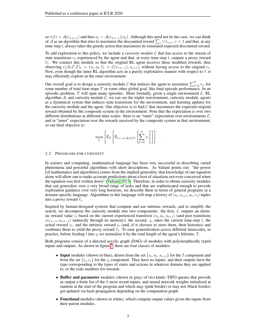
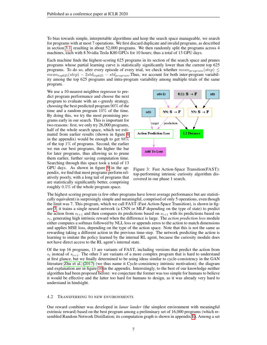
The highest scoring program (a few other programs have lower average performance but are statisti-
cally equivalent) is surprisingly simple and meaningful, comprised of only 5 operations, even though
the limit was 7. This program, which we call FAST (Fast Action-Space Transition), is shown in fig-
ure 3; it trains a single neural network (a CNN or MLP depending on the type of state) to predict
the action from st+1 and then compares its predictions based on st+1 with its predictions based on
st, generating high intrinsic reward when the difference is large. The action prediction loss module
either computes a softmax followed by NLL loss or appends zeros to the action to match dimensions
and applies MSE loss, depending on the type of the action space. Note that this is not the same as
rewarding taking a different action in the previous time-step. The network predicting the action is
learning to imitate the policy learned by the internal RL agent, because the curiosity module does
not have direct access to the RL agent’s internal state.
Of the top 16 programs, 13 are variants of FAST, including versions that predict the action from
st instead of st+1. The other 3 are variants of a more complex program that is hard to understand
at first glance, but we finally determined to be using ideas similar to cycle-consistency in the GAN
literature Zhu et al. (2017) (we thus name it Cycle-consistency intrinsic motivation); the diagram
and explanation are in figure 10 in the appendix. Interestingly, to the best of our knowledge neither
algorithm had been proposed before: we conjecture the former was too simple for humans to believe
it would be effective and the latter too hard for humans to design, as it was already very hard to
understand in hindsight.
Figure 3: Fast Action-Space Transition(FAST):
top-performing intrinsic curiosity algorithm dis-
covered in our phase 1 search.
4.2 TRANSFERRING TO NEW ENVIRONMENTS
Our reward combiner was developed in lunar lander (the simplest environment with meaningful
extrinsic reward) based on the best program among a preliminary set of 16,000 programs (which re-
sembled Random Network Distillation; its computation graph is shown in appendix E). Among a set
7
�
Published as a conference paper at ICLR 2020
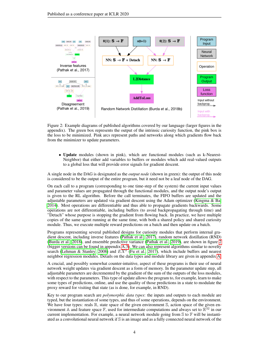
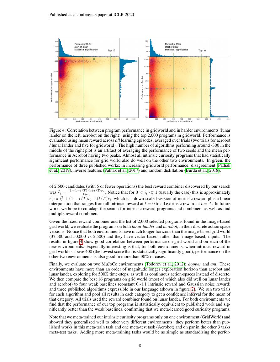
Figure 4: Correlation between program performance in gridworld and in harder environments (lunar
lander on the left, acrobot on the right), using the top 2,000 programs in gridworld. Performance is
evaluated using mean reward across all learning episodes, averaged over trials (two trials for acrobot
/ lunar lander and five for gridworld). The high number of algorithms performing around -300 in the
middle of the right plot is an artifact of averaging the performance of two seeds and the mean per-
formance in Acrobot having two peaks. Almost all intrinsic curiosity programs that had statistically
significant performance for grid world also do well on the other two environments. In green, the
performance of three published works; in increasing gridworld performance: disagreement (Pathak
et al., 2019), inverse features (Pathak et al., 2017) and random distillation (Burda et al., 2018).
1+it
was rt = (1+it−t/T )·it+t/T·rt
rt ≈ i2
of 2,500 candidates (with 5 or fewer operations) the best reward combiner discovered by our search
. Notice that for 0 < it 1 (usually the case) this is approximately
t + (1 − t/T )it + (t/T )rt, which is a down-scaled version of intrinsic reward plus a linear
interpolation that ranges from all intrinsic reward at t = 0 to all extrinsic reward at t = T . In future
work, we hope to co-adapt the search for intrinsic reward programs and combiners as well as find
multiple reward combiners.
Given the fixed reward combiner and the list of 2,000 selected programs found in the image-based
grid world, we evaluate the programs on both lunar lander and acrobot, in their discrete action space
versions. Notice that both environments have much longer horizons than the image-based grid world
(37,500 and 50,000 vs 2,500) and they have vector-based, rather than image-based, inputs. The
results in figure 4 show good correlation between performance on grid world and on each of the
new environments. Especially interesting is that, for both environments, when intrinsic reward in
grid world is above 400 (the lowest score that is statistically significantly good), performance on the
other two environments is also good in more than 90% of cases.
Finally, we evaluate on two MuJoCo environments (Todorov et al., 2012): hopper and ant. These
environments have more than an order of magnitude longer exploration horizon than acrobot and
lunar lander, exploring for 500K time-steps, as well as continuous action-spaces instead of discrete.
We then compare the best 16 programs on grid world (most of which also did well on lunar lander
and acrobot) to four weak baselines (constant 0,-1,1 intrinsic reward and Gaussian noise reward)
and three published algorithms expressible in our language (shown in figure 2). We run two trials
for each algorithm and pool all results in each category to get a confidence interval for the mean of
that category. All trials used the reward combiner found on lunar lander. For both environments we
find that the performance of our top programs is statistically equivalent to published work and sig-
nificantly better than the weak baselines, confirming that we meta-learned good curiosity programs.
Note that we meta-trained our intrinsic curiosity programs only on one environment (GridWorld) and
showed they generalized well to other very different environments: they perform better than pub-
lished works in this meta-train task and one meta-test task (Acrobot) and on par in the other 3 tasks
meta-test tasks. Adding more meta-training tasks would be as simple as standardising the perfor-
8
�


 2023年江西萍乡中考道德与法治真题及答案.doc
 2012年重庆南川中考生物真题及答案.doc
 2013年江西师范大学地理学综合及文艺理论基础考研真题.doc
 2020年四川甘孜小升初语文真题及答案I卷.doc
 2020年注册岩土工程师专业基础考试真题及答案.doc
 2023-2024学年福建省厦门市九年级上学期数学月考试题及答案.doc
 2021-2022学年辽宁省沈阳市大东区九年级上学期语文期末试题及答案.doc
 2022-2023学年北京东城区初三第一学期物理期末试卷及答案.doc
 2018上半年江西教师资格初中地理学科知识与教学能力真题及答案.doc
 2012年河北国家公务员申论考试真题及答案-省级.doc
 2020-2021学年江苏省扬州市江都区邵樊片九年级上学期数学第一次质量检测试题及答案.doc
 2022下半年黑龙江教师资格证中学综合素质真题及答案.doc