logo资料库

利用MATLAB和Excel 进行数值分析.pdf

第1页 / 共627页
第2页 / 共627页
第3页 / 共627页
第4页 / 共627页
第5页 / 共627页
第6页 / 共627页
第7页 / 共627页
第8页 / 共627页
资料共627页,剩余部分请下载后查看
Numerical Analysis Front Cover THIRD Edition.pdf
Numerical Analysis THIRD Edition Front Matter.pdf
Numerical Analysis THIRD Edition Preface.pdf
Numerical Analysis THIRD Edition TOC All Chapters.pdf
Numerical Analysis THIRD Edition Chapter 01.pdf
Chapter 1
1.1 Command Window
1.2 Roots of Polynomials
1.3 Polynomial Construction from Known Roots
1.4 Evaluation of a Polynomial at Specified Values
1.5 Rational Polynomials
1.6 Using MATLAB to Make Plots
1.7 Subplots
1.8 Multiplication, Division and Exponentiation
1.9 Script and Function Files
1.10 Display Formats
1.11 Summary
1.12 Exercises
1.13 Solutions to End-of-Chapter Exercises
Numerical Analysis THIRD Edition Chapter 02.pdf
Chapter 2
2.1 Newton’s Method for Root Approximation
2.2 Approximations with Spreadsheets
2.3 The Bisection Method for Root Approximation
2.4 Summary
2.5 Exercises
2.6 Solutions to End-of-Chapter Exercises
Numerical Analysis THIRD Edition Chapter 03.pdf
Chapter 3
3.1 Alternating Voltages and Currents
3.2 Characteristics of Sinusoids
3.3 Inverse Trigonometric Functions
3.4 Phasors
3.5 Addition and Subtraction of Phasors
3.6 Multiplication of Phasors
3.7 Division of Phasors
3.8 Exponential and Polar Forms of Phasors
3.9 Summary
3.10 Exercises
3.11 Solutions to End-of-Chapter Exercises
Numerical Analysis THIRD Edition Chapter 04.pdf
Chapter 4
4.1 Matrix Definition
4.2 Matrix Operations
4.3 Special Forms of Matrices
4.4 Determinants
4.5 Minors and Cofactors
4.6 Cramer’s Rule
4.7 Gaussian Elimination Method
4.8 The Adjoint of a Matrix
4.9 Singular and Non-Singular Matrices
4.10 The Inverse of a Matrix
4.11 Solution of Simultaneous Equations with Matrices
4.12 Summary
4.13 Exercises
4.14 Solutions to End-of-Chapter Exercises
Numerical Analysis THIRD Edition Chapter 05.pdf
Chapter 5
5.1 Simple Differential Equations
5.2 Classification
5.3 Solutions of Ordinary Differential Equations (ODE)
5.4 Solution of the Homogeneous ODE
5.5 Using the Method of Undetermined Coefficients for the Forced Response
5.6 Using the Method of Variation of Parameters for the Forced Response
5.7 Expressing Differential Equations in State Equation Form
5.8 Solution of Single State Equations
5.9 The State Transition Matrix
5.10 Computation of the State Transition Matrix
5.11 Eigenvectors
5.12 Summary
5.13 Exercises
5.14 Solutions to End-of-Chapter Exercises
Numerical Analysis THIRD Edition Chapter 06.pdf
Chapter 6
6.1 Wave Analysis
6.2 Evaluation of the Coefficients
6.3 Symmetry
6.4 Waveforms in Trigonometric Form of Fourier Series
6.5 Alternate Forms of the Trigonometric Fourier Series
6.6 The Exponential Form of the Fourier Series
6.7 Line Spectra
6.8 Numerical Evaluation of Fourier Coefficients
6.9 Power Series Expansion of Functions
6.10 Taylor and Maclaurin Series
6.11 Summary
6.12 Exercises
6.13 Solutions to End-of-Chapter Exercises
Numerical Analysis THIRD Edition Chapter 07.pdf
Chapter 7
7.1 Divided Differences
7.2 Factorial Polynomials
7.3 Antidifferences
7.4 Newton’s Divided Difference Interpolation Method
7.5 Lagrange’s Interpolation Method
7.6 Gregory-Newton Forward Interpolation Method
7.7 Gregory-Newton Backward Interpolation Method
7.8 Interpolation with MATLAB
7.9 Summary
7.10 Exercises
7.11 Solutions to End-of-Chapter Exercises
Numerical Analysis THIRD Edition Chapter 08.pdf
Chapter 8
8.1 Curve Fitting
8.2 Linear Regression
8.3 Parabolic Regression
8.4 Regression with Power Series Approximations
8.5 Summary
8.6 Exercises
8.7 Solutions to End-of-Chapter Exercises
Numerical Analysis THIRD Edition Chapter 09.pdf
Chapter 9
9.1 Taylor Series Method
9.2 Runge-Kutta Method
9.3 Adams’ Method
9.4 Milne’s Method
9.5 Summary
9.6 Exercises
9.7 Solutions to End-of-Chapter Exercises
Numerical Analysis THIRD Edition Chapter 10.pdf
Chapter 10
10.1 The Trapezoidal Rule
10.2 Simpson’s Rule
10.3 Summary
10.4 Exercises
10.5 Solution to End-of-Chapter Exercises
Numerical Analysis THIRD Edition Chapter 11.pdf
Chapter 11
11.1 Introduction
11.2 Definition, Solutions, and Applications
11.3 Fibonacci Numbers
11.4 Summary
11.5 Exercises
11.6 Solutions to End-of-Chapter Exercises
Numerical Analysis THIRD Edition Chapter 12.pdf
Chapter 12
12.1 Partial Fraction Expansion
12.2 Alternate Method of Partial Fraction Expansion
12.3 Summary
12.4 Exercises
12.5 Solutions to End-of-Chapter Exercises
Numerical Analysis THIRD Edition Chapter 13.pdf
Chapter 13
13.1 The Gamma Function
13.2 The Gamma Distribution
13.3 The Beta Function
13.4 The Beta Distribution
13.5 Summary
13.6 Exercises
13.7 Solutions to End-of-Chapter Exercises
Numerical Analysis THIRD Edition Chapter 14.pdf
Chapter 14
14.1 Orthogonal Functions
14.2 Orthogonal Trajectories
14.3 Orthogonal Vectors
14.4 The Gram-Schmidt Orthogonalization Procedure
14.5 The LU Factorization
14.6 The Cholesky Factorization
14.7 The QR Factorization
14.8 Singular Value Decomposition
14.9 Summary
14.10 Exercises
14.11 Solutions to End-of-Chapter Exercises
Numerical Analysis THIRD Edition Chapter 15.pdf
Chapter 15
15.1 The Bessel Function
15.2 Legendre Functions
15.3 Laguerre Polynomials
15.4 Chebyshev Polynomials
15.5 Summary
15.6 Exercises
15.7 Solutions to End-of-Chapter Exercises
Numerical Analysis THIRD Edition Chapter 16.pdf
Chapter 16
16.1 Linear Programming
16.2 Dynamic Programming
16.3 Network Analysis
16.4 Summary
16.5 Exercises
16.6 Solutions to End-of-Chapter Exercises
Numerical Analysis THIRD Edition Appendix A Difference Equations.pdf
Appendix A
A.1 Recursive Method for Solving Difference Equations
A.2 Method of Undetermined Coefficients
Numerical Analysis THIRD Edition Appendix B Introduction to Simulink.pdf
Appendix B
B.1 Simulink and its Relation to MATLAB
B.2 Simulink Demos
Numerical Analysis THIRD Edition Appendix C Ill-Conditioned Matrices.pdf
Appendix C
Ill-Conditioned Matrices
his appendix supplements Chapters 4 and 14 with concerns when the determinant of the coefficient matrix is small. We will introduce a reference against which the determinant can be measured to classify a matrix as a well- or ill-conditioned.
C.1 The Norm of a Matrix
A norm is a function which assigns a positive length or size to all vectors in a vector space, other than the zero vector. An example is the two-dimensional Euclidean space denoted as . The elements of the Euclidean vector space (e.g., (2,5))...
The Euclidean norm of a matrix , denoted as , is defined as
(C.1)
and it is computed with the MATLAB function norm(A).
Example C.1
Using the MATLAB function norm(A), compute the Euclidean norm of the matrix , defined as
Solution:
At the MATLAB command prompt, we enter
A=[-2 5 -4 9; -3 -6 8 1; 7 -5 3 2; 4 -9 -8 -1]; norm(A)
and MATLAB outputs
ans =
14.5539
C.2 Condition Number of a Matrix
The condition number of a matrix is defined as
(C.2)
where is the norm of the matrix defined in relation (C.1) above. Matrices with condition number close to unity are said to be well-conditioned matrices, and those with very large condition number are said to be ill-conditioned matrices.
The condition number of a matrix is computed with the MATLAB function cond(A).
Example C.2
Using the MATLAB function cond(A), compute the condition number of the matrix defined as
Solution:
At the MATLAB command prompt, we enter
A=[-2 5 -4 9; -3 -6 8 1; 7 -5 3 2; 4 -9 -8 -1]; cond(A)
and MATLAB outputs
ans =
2.3724
This condition number is relatively close to unity and thus we classify matrix A as a well-condi tioned matrix.
We recall from Chapter 4 that if the determinant of a square matrix A is singular, that is, if , the inverse of A is undefined. Please refer to Chapter 4, Page 4-22.
Now, let us consider that the coefficient matrix is very small, i.e., almost singular. Accordingly, we classify such a matrix as ill-conditioned.
C.3 Hilbert Matrices
Let be a positive integer. A unit fraction is the reciprocal of this integer, that is, . Thus, are unit fractions. A Hilbert matrix is a matrix with unit fraction elements
(C.3)
(C.4)
MATLAB’s function hilb(n) displays the Hilbert matrix.
Example C.3
Compute the determinant and the condition number of the Hilbert matrix using MATLAB.
Solution:
At the MATLAB command prompt, we enter
det(hilb(6))
and MATLAB outputs
ans =
5.3673e-018
This is indeed a very small number and for all practical purposes this matrix is singular.
We can find the condition number of a matrix A with the cond(A) MATLAB function. Thus, for the Hilbert matrix,
cond(hilb(6))
ans =
1.4951e+007
This is a large number and if the coefficient matrix is multiplied by this number, seven decimal places might be lost.
Let us consider another example.
Example C.4
Let where and
Compute the values of the vector .
Solution:
Here, we are asked to find the values of and of the linear system
Using MATLAB, we define and , and we use the left division operation, i.e.,
A=[0.585 0.378; 0.728 0.464]; b=[0.187 0.256]'; x=b\A
x =
2.9428 1.8852
Check:
A=[0.585 0.378; 0.728 0.464]; x=[2.9428 1.8852]'; b=A*x
b =
2.4341
3.0171
but these are not the given values of the vector , so let us check the determinant and the condi tion number of the matrix .
determinant = det(A)
determinant =
-0.0037
condition=cond(A)
condition =
328.6265
Therefore, we conclude that this system of equations is ill-conditioned and the solution is invalid.
Example C.4 above should serve as a reminder that when we solve systems of equations using matrices, we should check the determinants and the condition number to predict possible floating point and roundoff errors.
Numerical Analysis book Bibliography.pdf
References and Suggestions for Further Study
A. The following publications by The MathWorks, are highly recommended for further study. They are available from The MathWorks, 3 Apple Hill Drive, Natick, MA, 01760, www.mathworks.com.
1. Getting Started with MATLAB
2. Using MATLAB
3. Using MATLAB Graphics
4. Financial Toolbox
5. Statistics Toolbox
B. Other references indicated in footnotes throughout this text, are listed below.
1. Mathematics for Business, Science, and Technology with MATLAB and Excel Computations, Third Edition, ISBN-13: 978-1-934404-01-2
2. Circuit Analysis I with MATLAB Applications, ISBN 0-9709511-2-4
6. Handbook of Mathematical Functions, ISBN 0-4866127-2-4
7. CRC Standard Mathematical Tables, ISBN 0-8493-0626-4
Numerical Analysis, 3rd Edition Index All Chapters.pdf
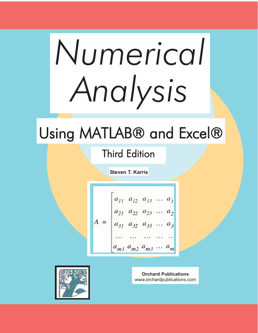
Numerical Analysis Using MATLAB® and Excel® Third Edition Steven T. Karris Orchard Publications www.orchardpublications.com
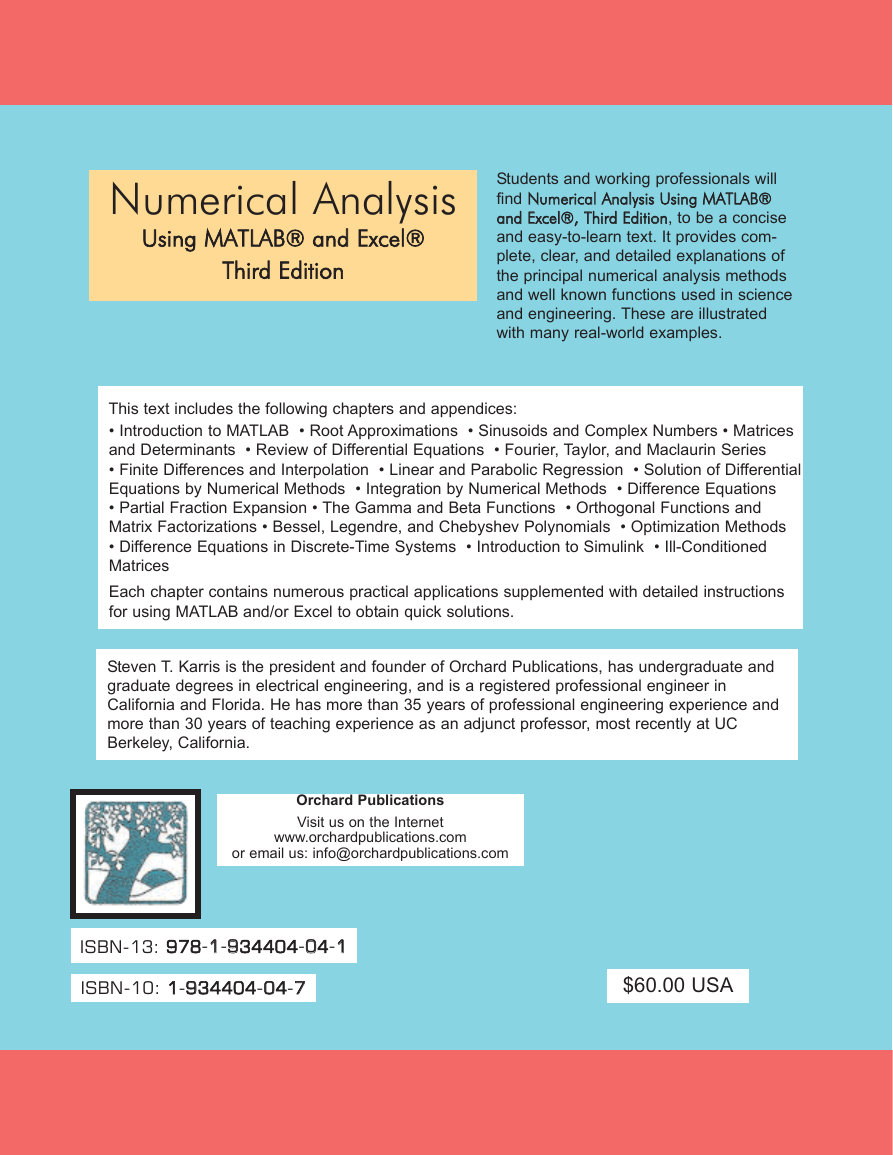
Numerical Analysis Using MATLAB® and Excel® Third Edition Students and working professionals will find NNuummeerriiccaall AAnnaallyyssiiss UUssiinngg MMAATTLLAABB®® aanndd EExxcceell®®,, TThhiirrdd EEddiittiioonn, to be a concise and easy-to-learn text. It provides com- plete, clear, and detailed explanations of the principal numerical analysis methods and well known functions used in science and engineering. These are illustrated with many real-world examples. This text includes the following chapters and appendices: • Introduction to MATLAB • Root Approximations • Sinusoids and Complex Numbers • Matrices and Determinants • Review of Differential Equations • Fourier, Taylor, and Maclaurin Series • Finite Differences and Interpolation • Linear and Parabolic Regression • Solution of Differential Equations by Numerical Methods • Integration by Numerical Methods • Difference Equations • Partial Fraction Expansion • The Gamma and Beta Functions • Orthogonal Functions and Matrix Factorizations • Bessel, Legendre, and Chebyshev Polynomials • Optimization Methods • Difference Equations in Discrete-Time Systems • Introduction to Simulink • Ill-Conditioned Matrices Each chapter contains numerous practical applications supplemented with detailed instructions for using MATLAB and/or Excel to obtain quick solutions. Steven T. Karris is the president and founder of Orchard Publications, has undergraduate and graduate degrees in electrical engineering, and is a registered professional engineer in California and Florida. He has more than 35 years of professional engineering experience and more than 30 years of teaching experience as an adjunct professor, most recently at UC Berkeley, California. Orchard Publications Visit us on the Internet www.orchardpublications.com or email us: info@orchardpublications.com ISBN-13: 978-11-9934404-004-11 ISBN-10: 1-9934404-004-77 $60.00 USA
Numerical Analysis Using MATLAB® and Excel® Third Edition Steven T. Karris Orchard Publications www.orchardpublications.com
Numerical Analysis Using MATLAB® and Excel®, Third Edition Copyright ” 2007 Orchard Publications. All rights reserved. Printed in the United States of America. No part of this publication may be reproduced or distributed in any form or by any means, or stored in a data base or retrieval system, without the prior written permission of the publisher. Direct all inquiries to Orchard Publications, info@orchardpublications.com Product and corporate names are trademarks or registered trademarks of the Microsoft™ Corporation and The MathWorks™, Inc. They are used only for identification and explanation, without intent to infringe. Library of Congress Cataloging-in-Publication Data Library of Congress Control Number: 2007922100 Copyright TX 5-589-152 ISBN-13: 978-1-934404-04-1 ISBN-10: 1-934404-04-7 Disclaimer The author has made every effort to make this text as complete and accurate as possible, but no warranty is implied. The author and publisher shall have neither liability nor responsibility to any person or entity with respect to any loss or damages arising from the information contained in this text.
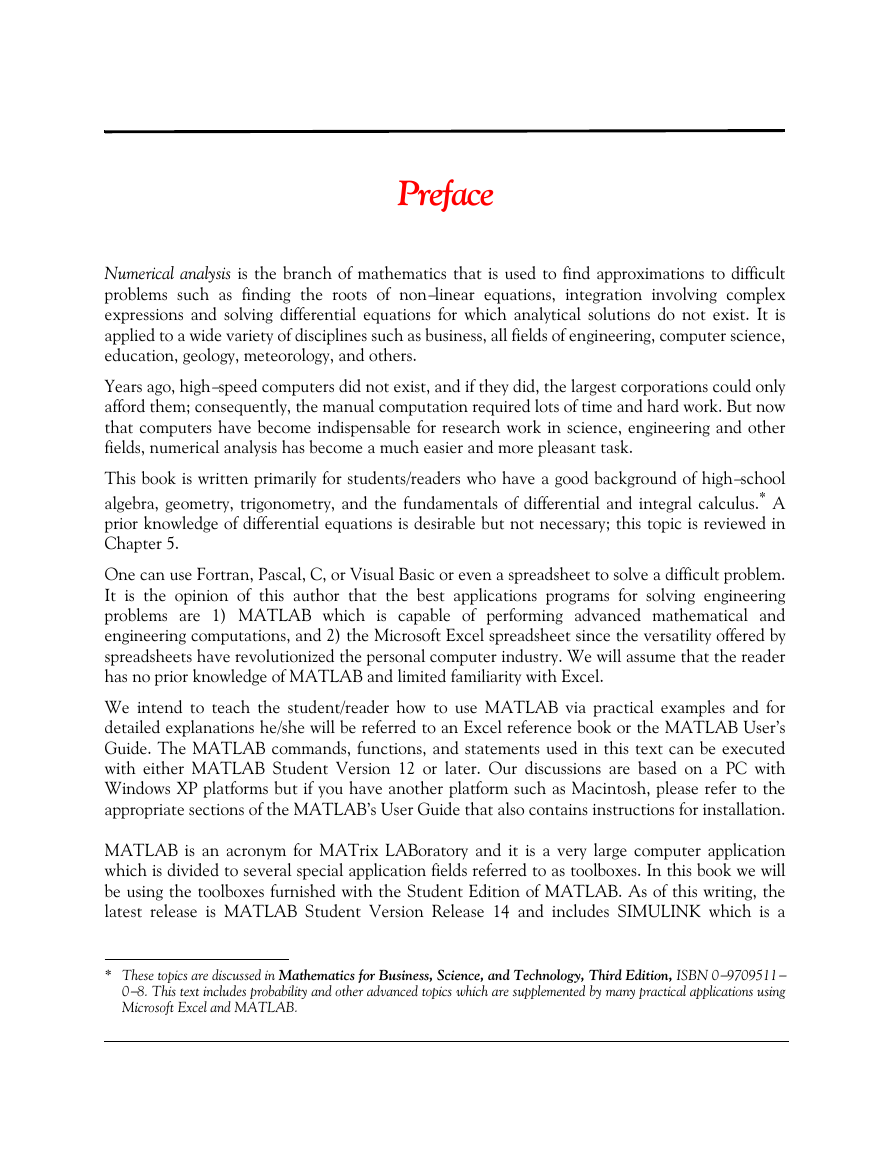
Preface Numerical analysis is the branch of mathematics that is used to find approximations to difficult problems such as finding the roots of non−linear equations, integration involving complex expressions and solving differential equations for which analytical solutions do not exist. It is applied to a wide variety of disciplines such as business, all fields of engineering, computer science, education, geology, meteorology, and others. Years ago, high−speed computers did not exist, and if they did, the largest corporations could only afford them; consequently, the manual computation required lots of time and hard work. But now that computers have become indispensable for research work in science, engineering and other fields, numerical analysis has become a much easier and more pleasant task. This book is written primarily for students/readers who have a good background of high−school algebra, geometry, trigonometry, and the fundamentals of differential and integral calculus.* A prior knowledge of differential equations is desirable but not necessary; this topic is reviewed in Chapter 5. One can use Fortran, Pascal, C, or Visual Basic or even a spreadsheet to solve a difficult problem. It is the opinion of this author that the best applications programs for solving engineering problems are 1) MATLAB which is capable of performing advanced mathematical and engineering computations, and 2) the Microsoft Excel spreadsheet since the versatility offered by spreadsheets have revolutionized the personal computer industry. We will assume that the reader has no prior knowledge of MATLAB and limited familiarity with Excel. We intend to teach the student/reader how to use MATLAB via practical examples and for detailed explanations he/she will be referred to an Excel reference book or the MATLAB User’s Guide. The MATLAB commands, functions, and statements used in this text can be executed with either MATLAB Student Version 12 or later. Our discussions are based on a PC with Windows XP platforms but if you have another platform such as Macintosh, please refer to the appropriate sections of the MATLAB’s User Guide that also contains instructions for installation. MATLAB is an acronym for MATrix LABoratory and it is a very large computer application which is divided to several special application fields referred to as toolboxes. In this book we will be using the toolboxes furnished with the Student Edition of MATLAB. As of this writing, the latest release is MATLAB Student Version Release 14 and includes SIMULINK which is a * These topics are discussed in Mathematics for Business, Science, and Technology, Third Edition, ISBN 0−9709511− 0−8. This text includes probability and other advanced topics which are supplemented by many practical applications using Microsoft Excel and MATLAB.
software package used for modeling, simulating, and analyzing dynamic systems. SIMULINK is not discussed in this text; the interested reader may refer to Introduction to Simulink with Engineering Applications, ISBN 0−9744239−7−1. Additional information including purchasing the software may be obtained from The MathWorks, Inc., 3 Apple Hill Drive, Natick, MA 01760−2098. Phone: 508 647−7000, Fax: 508 647−7001, e−mail: info@mathwork.com and web site http://www.mathworks.com. The author makes no claim to originality of content or of treatment, but has taken care to present definitions, statements of physical laws, theorems, and problems. Chapter 1 is an introduction to MATLAB. The discussion is based on MATLAB Student Version 5 and it is also applicable to Version 6. Chapter 2 discusses root approximations by numerical methods. Chapter 3 is a review of sinusoids and complex numbers. Chapter 4 is an introduction to matrices and methods of solving simultaneous algebraic equations using Excel and MATLAB. Chapter 5 is an abbreviated, yet practical introduction to differential equations, state variables, state equations, eigenvalues and eigenvectors. Chapter 6 discusses the Taylor and Maclaurin series. Chapter 7 begins with finite differences and interpolation methods. It concludes with applications using MATLAB. Chapter 8 is an introduction to linear and parabolic regression. Chapters 9 and 10 discuss numerical methods for differentiation and integration respectively. Chapter 11 is a brief introduction to difference equations with a few practical applications. Chapters 12 is devoted to partial fraction expansion. Chapters 13, 14, and 15 discuss certain interesting functions that find wide application in science, engineering, and probability. This text concludes with Chapter 16 which discusses three popular optimization methods. New to the Third Edition This is an extensive revision of the first edition. The most notable changes are the inclusion of Fourier series, orthogonal functions and factorization methods, and the solutions to all end−of− chapter exercises. It is in response to many readers who expressed a desire to obtain the solutions in order to check their solutions to those of the author and thereby enhancing their knowledge. Another reason is that this text is written also for self−study by practicing engineers who need a review before taking more advanced courses such as digital image processing. The author has prepared more exercises and they are available with their solutions to those instructors who adopt this text for their class. Another change is the addition of a rather comprehensive summary at the end of each chapter. Hopefully, this will be a valuable aid to instructors for preparation of view foils for presenting the material to their class. The last major change is the improvement of the plots generated by the latest revisions of the MATLAB® Student Version, Release 14. Orchard Publications Fremont, California www.orchardpublications.com info@orchardpublications.com
Table of Contents 1 Introduction to MATLAB 1−1 1.1 Command Window.................................................................................................1−1 1.2 Roots of Polynomials...............................................................................................1−3 1.3 Polynomial Construction from Known Roots ........................................................1−4 1.4 Evaluation of a Polynomial at Specified Values .....................................................1−5 1.5 Rational Polynomials ..............................................................................................1−8 1.6 Using MATLAB to Make Plots..............................................................................1−9 1.7 Subplots.................................................................................................................1−18 1.8 Multiplication, Division and Exponentiation.......................................................1−19 1.9 Script and Function Files......................................................................................1−26 1.10 Display Formats ....................................................................................................1−31 1.11 Summary ...............................................................................................................1−33 1.12 Exercises................................................................................................................1−37 1.13 Solutions to End−of−Chapter Exercises ...............................................................1−38 MATLAB Computations: Entire chapter 2 Root Approximations 2−1 2.1 Newton’s Method for Root Approximation...........................................................2−1 2.2 Approximations with Spreadsheets........................................................................2−7 2.3 The Bisection Method for Root Approximation .................................................2−19 2.4 Summary...............................................................................................................2−27 2.5 Exercises ...............................................................................................................2−28 2.6 Solutions to End−of−Chapter Exercises...............................................................2−29 MATLAB Computations: Pages 2−2 through 2−7, 2−14, 2−21 through 2−23, 2−29 through 2−34 Excel Computations: Pages 2−8 through 2−19, 2−24 through 2−26 3 Sinusoids and Phasors 3−1 3.1 Alternating Voltages and Currents ........................................................................3−1 3.2 Characteristics of Sinusoids....................................................................................3−2 Inverse Trigonometric Functions .........................................................................3−10 3.3 3.4 Phasors..................................................................................................................3−10 3.5 Addition and Subtraction of Phasors ...................................................................3−11 3.6 Multiplication of Phasors......................................................................................3−12 3.7 Division of Phasors ...............................................................................................3−13 Numerical Analysis Using MATLAB® and Excel®, Third Edition Copyright © Orchard Publications i
3.8 Exponential and Polar Forms of Phasors ..............................................................3−13 3.9 Summary ...............................................................................................................3−24 3.10 Exercises................................................................................................................3−27 3.11 Solutions to End−of−Chapter Exercises................................................................3−28 MATLAB Computations: Pages 3−15 through 3−23, 3−28 through 3−31 Simulink Modeling: Pages 3−16 through 3−23 4 Matrices and Determinants 4−1 4.1 Matrix Definition.....................................................................................................4−1 4.2 Matrix Operations ...................................................................................................4−2 4.3 Special Forms of Matrices........................................................................................4−5 4.4 Determinants...........................................................................................................4−9 4.5 Minors and Cofactors ............................................................................................4−13 4.6 Cramer’s Rule ........................................................................................................4−18 4.7 Gaussian Elimination Method...............................................................................4−20 4.8 The Adjoint of a Matrix ........................................................................................4−22 4.9 Singular and Non−Singular Matrices ....................................................................4−22 4.10 The Inverse of a Matrix.........................................................................................4−23 4.11 Solution of Simultaneous Equations with Matrices ..............................................4−25 4.12 Summary................................................................................................................4−32 4.13 Exercises ................................................................................................................4−36 4.14 Solutions to End−of−Chapter Exercises ................................................................4−38 MATLAB Computations: Pages 4−3, 4−5 through 4−8, 4−10, 4−12, 4−3, 4−5, 4−19 through 4−20, 4−24, 4−26, 4−28, 4−30, 4−38, 4−41, 4−43 Excel Computations: Pages 4−28 through 4−29, 4−42 through 4−43 5 Differential Equations, State Variables, and State Equations 5−1 5.1 Simple Differential Equations..................................................................................5−1 5.2 Classification............................................................................................................5−2 5.3 Solutions of Ordinary Differential Equations (ODE) .............................................5−6 5.4 Solution of the Homogeneous ODE ...................................................................... 5−8 5.5 Using the Method of Undetermined Coefficients for the Forced Response........ 5−10 5.6 Using the Method of Variation of Parameters for the Forced Response ............. 5−20 5.7 Expressing Differential Equations in State Equation Form.................................. 5−24 5.8 Solution of Single State Equations....................................................................... 5−27 5.9 The State Transition Matrix ................................................................................ 5−28 5.10 Computation of the State Transition Matrix...................................................... 5−30 5.11 Eigenvectors.......................................................................................................... 5−38 5.12 Summary.............................................................................................................. 5−42 ii Numerical Analysis Using MATLAB® and Excel®, Third Edition Copyright © Orchard Publications
分享到:
收藏