Appendix A: Component Software Architecture 1 Introduction We outline the design of a component-based software architecture that analyses and val- ues industrial investment projects. We use the contingent claim, or real option, valuation method, which views a project as a claim to future cash flows which are dependent on un- derlying stochastic factors, such as the market price of a produced commodity. The software architecture enables the user to use domain and mathematical level constructs to specify the nature of the project and the stochastic behaviour of underlying factors. Meaning pre- serving symbolic rewrite rules transform these specifications into problem representations that are suitable for numerical solution. The transformed problem representations are then combined with components implementing parallel algorithms in order to compute solutions. The aim of this approach is to benefit strategic industrial decision-making by enabling high-level and flexible problem formulation and by using high performance computational resources. 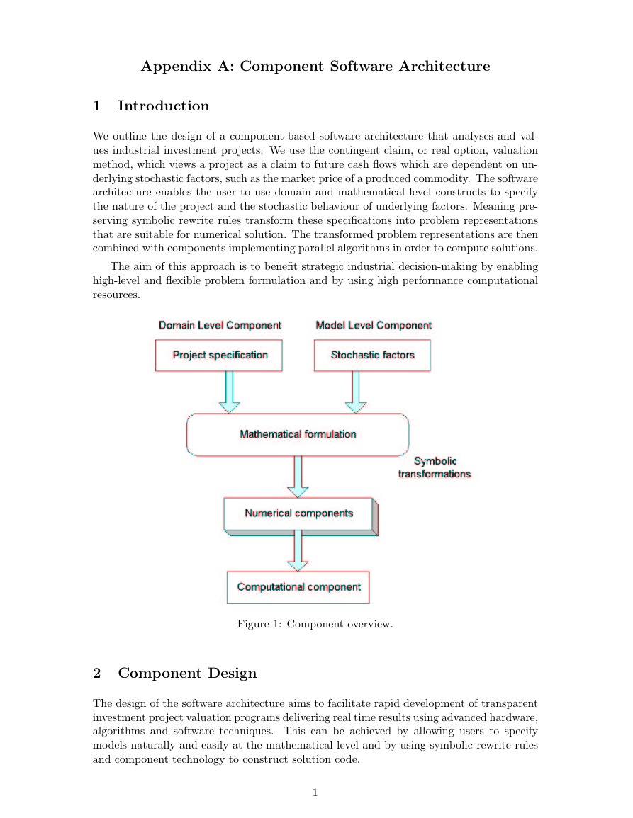Figure 1: Component overview. 2 Component Design The design of the software architecture aims to facilitate rapid development of transparent investment project valuation programs delivering real time results using advanced hardware, algorithms and software techniques. This can be achieved by allowing users to specify models naturally and easily at the mathematical level and by using symbolic rewrite rules and component technology to construct solution code. 1 

In order to structure solution code we generate components representing views of the problem at different levels of abstraction: the domain level, the model level and the numer- ical level. These are combined using software -mechanisms of inheritance and composition to produce the final computational component, which actually computes the solution. Such an approach aims to retain high level information and facilitate component re-use and hence problem reformulation. 3 Domain Level Component The basis for valuing investment projects are the streams of uncertain cash flows the project produces. A symbolic language specifies investment projects and underlying factor models. This comprises equations specifying cash flows contingent on system variables and stochas- tic equations modelling system variables. The basic equation defining the project is the profit function simply defined as revenue minus costs. For a specific project the individual components of revenue and costs are specified. Thus at the domain level the user specifies the project in terms of its contingent cash flows. These define the profit function, which is a function of time, the decision variables of the project management, and the random underlying factors. This specification can be made using structured text, such as XML. Alternatively the specification could be made using a symbolic programming language such as Mathematica or Maple, which would fa- cilitate the symbolic transformations described below. In either case the specification can then be automatically processed to construct a C++ component representing the project. This enables its reuse in the specification of future problems and provides a (domain-level) symbolic name for its structure. These components define projects abstractly by defining the types’ permitted opera- tions; thus they provide an external interface to the computational derivative components which are subtypes. This facilitates polymorphism so that model and numerical components can be modified without disruption to client applications. Each component has as its data members the specified decision variables, the random underlying factors and as member function the profit function. Note that at this point we have not yet defined the stochastic behaviour. This is because often the user may wish to try out various different stochastic models, and over time may change his or her view of which model is most appropriate. The domain level C++ component is independent of model, and thus need not change when the model or its numerical implementation changes. 4 Model Level Component Any realistic model of an industrial project involves uncertainties. For example, the future demand of a commodity, the price of raw materials, government policy on pollution, all are to a greater or lesser extent unknown. These factors which are uncertain are modelled as stochastic factors. The dynamics of the stochastic factors are specified as stochastic processes. These can be in discrete time or in continuous time, in which case they can be specified as stochastic differential equations (SDEs) which allow the specification of very general stochastic pro- cesses and admit a simple intuitive interpretation: The movement over time of the process is composed of two parts: a deterministic drift and a random diffusion, which is driven by a standard Brownian motion. We employ symbolic programming language to specify such 2 

SDEs as triples of the form: name,drift,diffusion. Once the model is represented in this way we can apply symbolic transformations written in the symbolic language. For example we have writtten a symbolic analytical solver for simple SDEs (linear or reducible to linear form). Further symbolic transformations encode results from stochastic analysis, such as: 1. the Ito formula, which gives the SDE for a functional of an SDE 2. Girsanov’s theorem, which gives the SDE for a process under a change of probability measure (which is fundamental to contingent claim theory). 3. The differential generator of an SDE, which is a partial differentail operator which can be used to contruct related partial differential equations, such as Kolmogorov’s equations and contingnent claim pricing equations such as Black-Scholes type equa- tions In short the model component contains the specification of the dynamics of relevant stochas- tic factors , and also further information derived from the specifications using symbolic transformations. This information is held in the symbolic programming language file, and also can be translated into a C++ model component. 5 Symbolic Transformations and Problem Representation The domain level and model level components together give a software representation of the mathematical problem definition, which is in general a stochastic control problem. Further symbolic transformations can be applied to simplify or reformulate this representation. For example we can encode the algebraic properties of the expectation operator, such as linearity and idempotency, as rewrite rules. Such rewrite rules take the form of: ⇒ aE[X] E[aX] E[X + Y ] ⇒ E[X] + E[X] E[E[X]] ⇒ E[X] Applying these rewrite rules to the symbolic software representation of the mathematical problem, we can derive expressions for the mean, variance and higher-order moments of the objective function. Since these expressions can become very complicated, this automatic derivation eliminates possibilities of human error. The advantage of using symbolic transformations of specifications to provide different representations is that the meaning of the program is given by the specification and is preserved by the transformations. However, efficient implementation is achieved by using pre-existing components for the implementation of numerical solution. Thus this approach utilises separation of program meaning and program implementation which potentially can facilitate a high level programming approach with efficient implementation. 6 Numerical Level Component Algorithms that solve the types of problems encountered are encapsulated in numerical components. We plan to re-use or repackage existing algorithmic code, or to write new numerical components for novel algorithms. 3 

Since the general stochastic control problem can be represented in various ways, de- pending on the properties of the specific problem, there exists a wide variety of numerical methods that can be used to solve the differing representations. When posed in continuous time the stochastic control problem can often be stated more explicitly as a non-linear Hamilton-Jacobi-Bellman equation. Such a representation can be solved using finite difference or spectral methods. Explicit finite difference methods can be effectively parallelised by decomposing the spatial domain and using a halo for local boundary communication. However the stability conditions can be very restrictive on the relative sizes of time and spatial steps. Implicit finite difference methods involve the solution of a matix equation at each step and there exist many effective ways to parallelise direct or iterative solutions. When decision boundaries can be computed a priori, for example when the stochastic control problem involves only open loop controls (see Intriligator), simulation methods can be used to compute solutions. By their nature Monte Carlo simulation methods parallelise very easily and effectively. When this is not the case i.e. when the optimal decisions are functions of time and the state variables and must be computed along with the overall solution (closed loop controls), dynamic programming methods are useful. For details of initial implementation of parallel dynamic programming methods on a lattice see Tsang. Finally in some cases the stochastic control problem can be transformed into a deter- ministic control or optimistation problem. Then methods such as dynamic programming, the simplex method, and Newtonian methods can be utilised. We have constructed parallel algorithm components suited to the solution of the contin- gent claims problems by writing Single Program Multiple Data parallel code using MPI and using SPRNG for parallel random number generation. In the future we intend to construct parallel algorithm components exculsively around existing high performance libraries, such as SPRNG and SCALAPACK. 7 Computational Component A computational component that actually solves the problem is constructed by combining information from the domain level and model level components with numerical compo- nents. The object-oriented mechanism of class inheritance and composition can facilitate this combining of information: the computational component can inherit from both the domain level and model level component in order to contain the project profit function and symbolically derived model information, such as analytical SDE solutions and alter- native mathematical problem definitions. The numerical component appropriate to the representation symbolically derived in the model component can then be called, taking as a parameter the relevant information from the domain and model level components. Such a software design aims to facilitate the rapid construction of programs using alter- native algorithms by re-using existing domain level and model level components. A similar software architecture was successfully applied to financial option problems in Automatic Generation of Software Components for Financial Modelling [Bunnin]. References [1] Blackford L.S, J. Choi, A. Cleary, E. D’Azevedo, J. Demmel, I. Dhillon, J. Dongarra, S. Hammarling, G. Henry, A. Petitet, K. Stanley, D. Walker, R. C. Whaley, ScaLAPACK 4 

User’s Guide http://netlib2.cs.utk.edu/scalapack/slug/scalapack slug.html 1997. [2] Cyganowski S., A Maple package for Stochastic Differential Equations, in Compu- tational Techniques ans Applications 1996 eds A. Easton, R. May Singapore World Scientific. [3] Cyganowski S., Solving Stochastic Differential Equations with Maple, http://net.indra.com/ sullivan/q253.html. [4] Darlington J., Guo Y., To H.W., Yang J., Functional Skeletons for Parallel Coordi- nation, in Haridi S., Ali K, Magnusson P. eds Proceedings of Europar 95, Springer August 1995. [5] Intriligator M.D., Mathematical Optimisation and Economic Theory, Prentice Hall 1971. [6] Kant E., C. Randall, A. Chhabra, Using Program Synthesis to Price Derivatives, Journal of Computational Finance vol. 1 no. 2 (Winter 1997/98) 97-129. [7] Tsang Mang Kin, Frdrick, Using Multiprocessors for Pricing American Options, MSc thesis, Dept. of Computing, Imperial College 2000. 5