Mining Association Rules between Sets of Items in Large Databases
Rakesh Agrawal
Tomasz Imielinski
Arun Swami
IBM Almaden Research Center
��� Harry Road, San Jose, CA ����
Abstract
We are given a large database of customer transactions.
Each transaction consists of items purchased by a customer
in a visit. We present an ecient algorithm that generates all
signicant association rules between items in the database.
The algorithm incorporates buer management and novel
estimation and pruning techniques. We also present results
of applying this algorithm to sales data obtained from a
large retailing company, which shows the eectiveness of the
algorithm.
� Introduction
Consider a supermarket with a large collection of items.
Typical business decisions that the management of the
supermarket has to make include what to put on sale,
how to design coupons, how to place merchandise on
shelves in order to maximize the prot, etc. Analysis
of past transaction data is a commonly used approach
in order to improve the quality of such decisions.
Until recently, however, only global data about the
cumulative sales during some time period (a day, a week,
a month, etc.) was available on the computer. Progress
in bar-code technology has made it possible to store the
so called basket data that stores items purchased on a
per-transaction basis. Basket data type transactions do
not necessarily consist of items bought together at the
same point of time. It may consist of items bought by
a customer over a period of time. Examples include
monthly purchases by members of a book club or a
music club.
Current address: Computer Science Department, Rutgers
University, New Brunswick, NJ �� ��
Permission to copy without fee all or part of this
material is granted provided that the copies are not made
or distributed for direct commercial advantage, the ACM
copyright notice and the title of the publication and its date
appear, and notice is given that copying is by permission
of the Association for Computing Machinery. To copy
otherwise, or to republish, requires a fee and/or special
permission.
Proceedings of the � � ACM SIGMOD Conference
Washington DC, USA, May � �
Several organizations have collected massive amounts
of such data. These data sets are usually stored
on tertiary storage and are very slowly migrating to
database systems. One of the main reasons for the
limited success of database systems in this area is
that current database systems do not provide necessary
functionality for a user interested in taking advantage
of this information.
This paper introduces the problem of \mining" a large
collection of basket data type transactions for associa-
tion rules between sets of items with some minimum
specied condence, and presents an ecient algorithm
for this purpose. An example of such an association rule
is the statement that �% of transactions that purchase
bread and butter also purchase milk. The antecedent
of this rule consists of bread and butter and the con-
sequent consists of milk alone. The number �% is the
condence factor of the rule.
The work reported in this paper could be viewed as a
step towards enhancing databases with functionalities
to process queries such as (we have omitted the
condence factor specication):
Find all rules that have \Diet Coke" as consequent.
These rules may help plan what the store should do
to boost the sale of Diet Coke.
Find all rules that have \bagels" in the antecedent.
These rules may help determine what products may
be impacted if the store discontinues selling bagels.
Find all rules that have \sausage" in the antecedent
and \mustard" in the consequent. This query can be
phrased alternatively as a request for the additional
items that have to be sold together with sausage in
order to make it highly likely that mustard will also
be sold.
Find all the rules relating items located on shelves
A and B in the store. These rules may help shelf
planning by determining if the sale of items on shelf
A is related to the sale of items on shelf B.
�
�
Find the \best" k rules that have \bagels" in the
consequent. Here, \best" can be formulated in terms
of the condence factors of the rules, or in terms
of their support,
i.e., the fraction of transactions
satisfying the rule.
The organization of the rest of the paper is as
In Section �, we give a formal statement of
follows.
the problem.
In Section �, we present our algorithm
for mining association rules. In Section �, we present
some performance results showing the eectiveness of
our algorithm, based on applying this algorithm to data
from a large retailing company. In Section �, we discuss
related work. In particular, we put our work in context
with the rule discovery work in AI. We conclude with a
summary in Section �.
� Formal Model
Let I = I�; I�; . . . ; Im be a set of binary attributes,
called items. Let T be a database of transactions. Each
transaction t is represented as a binary vector, with t[k]
= � if t bought the item Ik, and t[k] = � otherwise.
There is one tuple in the database for each transaction.
Let X be a set of some items in I. We say that a
transaction t satises X if for all items Ik in X, t[k] =
�.
By an association rule, we mean an implication of the
form X =) Ij, where X is a set of some items in I, and
Ij is a single item in I that is not present in X. The
rule X =) Ij is satised in the set of transactions T
with the condence factor � c � i at least c% of
transactions in T that satisfy X also satisfy Ij. We will
use the notation X =) Ij j c to specify that the rule
X =) Ij has a condence factor of c.
Given the set of transactions T , we are interested
in generating all rules that satisfy certain additional
constraints of two dierent forms:
�. Syntactic Constraints: These constraints involve
restrictions on items that can appear in a rule. For
example, we may be interested only in rules that have
a specic item Ix appearing in the consequent, or
rules that have a specic item Iy appearing in the
antecedent. Combinations of the above constraints
are also possible | we may request all rules that have
items from some predened itemset X appearing in
the consequent, and items from some other itemset
Y appearing in the antecedent.
�. Support Constraints: These constraints concern the
number of transactions in T that support a rule. The
support for a rule is dened to be the fraction of
transactions in T that satisfy the union of items in
the consequent and antecedent of the rule.
Support should not be confused with condence.
While condence is a measure of the rule’s strength,
support corresponds to statistical signicance.
Besides statistical signicance, another motivation
for support constraints comes from the fact that
we are usually interested only in rules with support
above some minimum threshold for business reasons.
If the support is not large enough, it means that the
rule is not worth consideration or that it is simply
less preferred (may be considered later).
In this formulation, the problem of rule mining can
be decomposed into two subproblems:
�. Generate all combinations of items that have frac-
tional transaction support above a certain thresh-
old, called minsupport. Call those combinations large
itemsets, and all other combinations that do not meet
the threshold small itemsets.
Syntactic constraints further constrain the admissible
combinations. For example, if only rules involving an
item Ix in the antecedent are of interest, then it is
sucient to generate only those combinations that
contain Ix.
�. For a given large itemset Y = I�I� . . . Ik, k �,
generate all rules (at the most k rules) that use items
from the set I�; I�; . . . ; Ik. The antecedent of each
of these rules will be a subset X of Y such that
X has k � items, and the consequent will be the
item Y X. To generate a rule X =) Ij j c,
where X = I�I� . . . Ij�Ij+� . . . Ik, take the support
of Y and divide it by the support of X. If the ratio
is greater than c then the rule is satised with the
condence factor c; otherwise it is not.
Note that if the itemset Y is large, then every subset
of Y will also be large, and we must have available
their support counts as the result of the solution of
the rst subproblem. Also, all rules derived from
Y must satisfy the support constraint because Y
satises the support constraint and Y is the union
of items in the consequent and antecedent of every
such rule.
Having determined the large itemsets, the solution
to the second subproblem is rather straightforward. In
the next section, we focus on the rst subproblem. We
develop an algorithm that generates all subsets of a
given set of items that satisfy transactional support
requirement. To do this task eciently, we use some
estimation tools and some pruning techniques.
� Discovering large itemsets
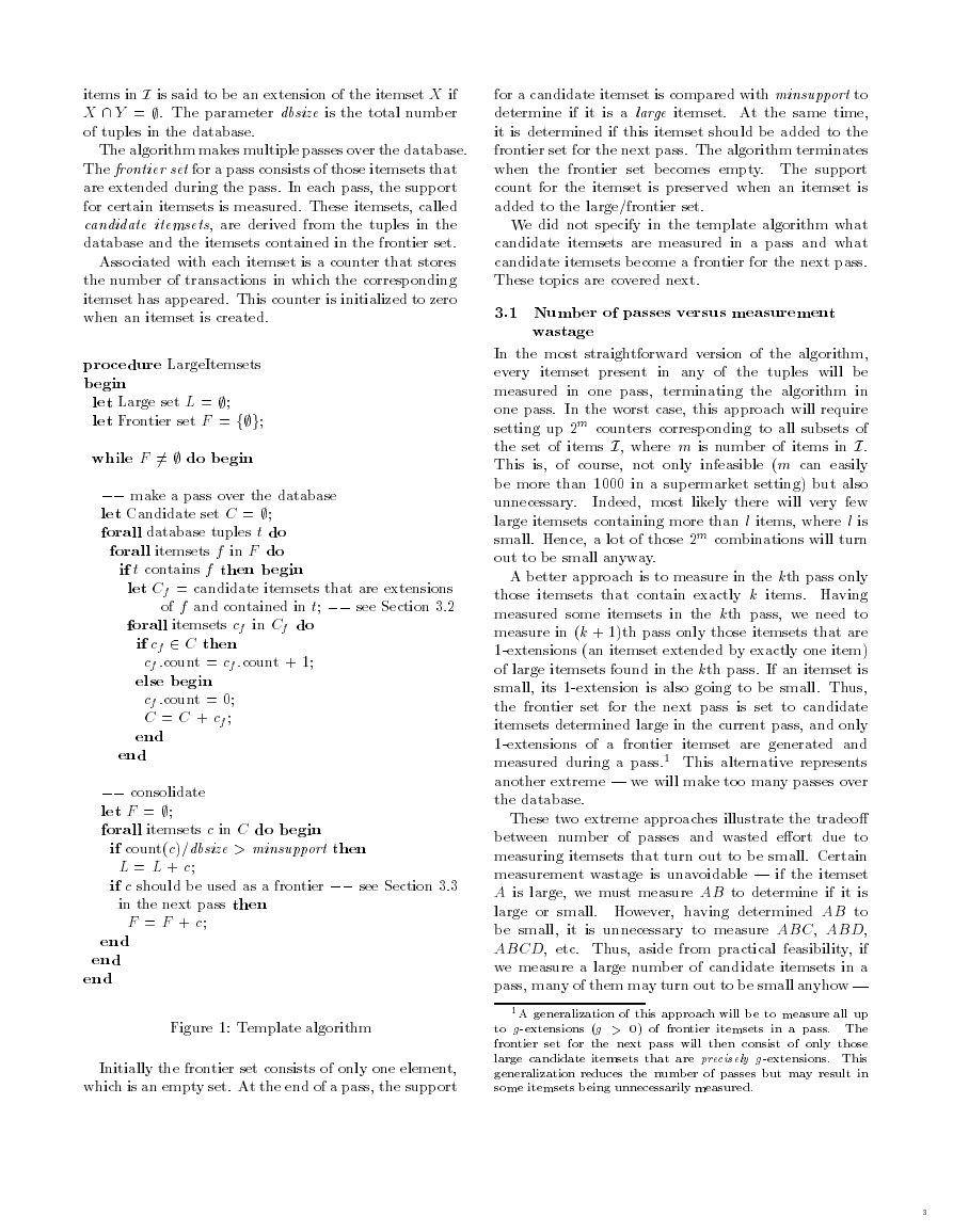
Figure � shows the template algorithm for nding large
itemsets. Given a set of items I, an itemset X + Y of
�
�
items in I is said to be an extension of the itemset X if
X \ Y = ;. The parameter dbsize is the total number
of tuples in the database.
The algorithm makes multiple passes over the database.
The frontier set for a pass consists of those itemsets that
are extended during the pass. In each pass, the support
for certain itemsets is measured. These itemsets, called
candidate itemsets, are derived from the tuples in the
database and the itemsets contained in the frontier set.
Associated with each itemset is a counter that stores
the number of transactions in which the corresponding
itemset has appeared. This counter is initialized to zero
when an itemset is created.
procedure LargeItemsets
begin
let Large set L = ;;
let Frontier set F = f;g;
while F �= ; do begin
make a pass over the database
let Candidate set C = ;;
forall database tuples t do
forall itemsets f in F do
if t contains f then begin
let Cf = candidate itemsets that are extensions
of f and contained in t; see Section �.�
forall itemsets cf in Cf do
if cf � C then
cf .count = cf .count + �;
else begin
cf .count = �;
C = C + cf ;
end
end
consolidate
let F = ;;
forall itemsets c in C do begin
if count(c)/dbsize > minsupport then
L = L + c;
if c should be used as a frontier see Section �.�
in the next pass then
F = F + c;
end
end
end
Figure �: Template algorithm
Initially the frontier set consists of only one element,
which is an empty set. At the end of a pass, the support
for a candidate itemset is compared with minsupport to
determine if it is a large itemset. At the same time,
it is determined if this itemset should be added to the
frontier set for the next pass. The algorithm terminates
when the frontier set becomes empty. The support
count for the itemset is preserved when an itemset is
added to the large/frontier set.
We did not specify in the template algorithm what
candidate itemsets are measured in a pass and what
candidate itemsets become a frontier for the next pass.
These topics are covered next.
�.� Number of passes versus measurement
wastage
In the most straightforward version of the algorithm,
every itemset present in any of the tuples will be
measured in one pass, terminating the algorithm in
one pass. In the worst case, this approach will require
setting up �m counters corresponding to all subsets of
the set of items I, where m is number of items in I.
This is, of course, not only infeasible (m can easily
be more than ���� in a supermarket setting) but also
unnecessary.
Indeed, most likely there will very few
large itemsets containing more than l items, where l is
small. Hence, a lot of those �m combinations will turn
out to be small anyway.
A better approach is to measure in the kth pass only
those itemsets that contain exactly k items. Having
measured some itemsets in the kth pass, we need to
measure in (k + �)th pass only those itemsets that are
�-extensions (an itemset extended by exactly one item)
of large itemsets found in the kth pass. If an itemset is
small, its �-extension is also going to be small. Thus,
the frontier set for the next pass is set to candidate
itemsets determined large in the current pass, and only
�-extensions of a frontier itemset are generated and
measured during a pass.� This alternative represents
another extreme | we will make too many passes over
the database.
These two extreme approaches illustrate the tradeo
between number of passes and wasted eort due to
measuring itemsets that turn out to be small. Certain
measurement wastage is unavoidable | if the itemset
A is large, we must measure AB to determine if it is
large or small. However, having determined AB to
be small, it is unnecessary to measure ABC, ABD,
ABCD, etc. Thus, aside from practical feasibility, if
we measure a large number of candidate itemsets in a
pass, many of them may turn out to be small anyhow |
�A generalization of this approach will be to measure all up
to g-extensions (g > �) of frontier itemsets in a pass. The
frontier set for the next pass will then consist of only those
large candidate itemsets that are precisely g-extensions. This
generalization reduces the number of passes but may result in
some itemsets being unnecessarily measured.
�
�
wasted eort. On the other hand, if we measure a small
number of candidates and many of them turn out to be
large then we need another pass, which may have not
been necessary. Hence, we need some careful estimation
before deciding whether a candidate itemset should be
measured in a given pass.
�.� Determination of candidate itemsets
One may think that we should measure in the current
pass only those extensions of frontier itemsets that are
expected to be large. However, if it were the case and
the data behaved according to our expectations and the
itemsets expected to be large indeed turn out to be
large, then we would still need another pass over the
database to determine the support of the extensions of
those large itemsets. To avoid this situation, in addition
to those extensions of frontier itemsets that are expected
to be large, we also measure the extensions X + Ij that
are expected to be small but such that X is expected
to be large and X contains a frontier itemset. We do
not, however, measure any further extensions of such
itemsets. The rationale for this choice is that if our
predictions are correct and X + Ij indeed turns out to
be small then no superset of X + Ij has to be measured.
The additional pass is then needed only if the data does
not behave according to our expectation and X + Ij
turns out to be large. This is the reason why not
measuring X + Ij that are expected to be small would
be a mistake | since even when the data agrees with
predictions, an extra pass over the database would be
necessary.
Expected support for an itemset
We use the statistical
independence assumption to
estimate the support for an itemset. Suppose that a
candidate itemset X + Y is a k-extension of the frontier
itemset X and that Y = I�I� . . . Ik. Suppose that the
itemset X appears in a total of x tuples. We know
the value of x since X was measured in the previous
pass (x is taken to be dbsize for the empty frontier
itemset). Suppose that X + Y is being considered as
a candidate itemset for the rst time after c tuples
containing X have already been processed in the current
pass. Denoting by f(Ij ) the relative frequency of the
item Ij in the database, the expected support s for the
itemset X + Y is given by
s = f (I�) f (I�) . . . f(Ik) (x c)=dbsize
Note that (x c)=dbsize is the actual support for X in
the remaining portion of the database. Under statistical
independence assumption, the expected support for X +
Y is a product of the support for X and individual
relative frequencies of items in Y .
If s is less than minsupport, then we say that X + Y
is expected to be small; otherwise, it is expected to be
large.
Candidate itemset generation procedure
An itemset not present in any of the tuples in the
database never becomes a candidate for measurement.
We read one tuple at a time from the database and
check what frontier sets are contained in the tuple read.
Candidate itemsets are generated from these frontier
itemset by extending them recursively with other items
present in the tuple. An itemset that is expected to be
small is not further extended. In order not to replicate
dierent ways of constructing the same itemset, items
are ordered and an itemset X is tried for extension only
by items that are later in the ordering than any of the
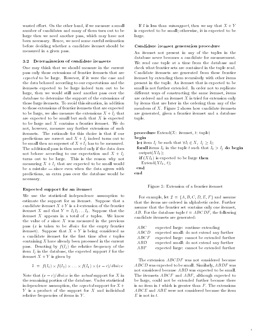
members of X. Figure � shows how candidate itemsets
are generated, given a frontier itemset and a database
tuple.
procedure Extend(X: itemset, t: tuple)
begin
let item Ij be such that �Il � X; Ij Il;
forall items Ik in the tuple t such that Ik > Ij do begin
output(XIk);
if (XIk) is expected to be large then
Extend(XIk , t);
end
end
Figure �: Extension of a frontier itemset
For example, let I = fA; B; C; D; E; F g and assume
that the items are ordered in alphabetic order. Further
assume that the frontier set contains only one itemset,
AB. For the database tuple t = ABCDF , the following
candidate itemsets are generated:
expected large: continue extending
ABC
ABCD expected small: do not extend any further
expected large: cannot be extended further
ABCF
expected small: do not extend any further
ABD
ABF
expected large: cannot be extended further
The extension ABCDF was not considered because
ABCD was expected to be small. Similarly, ABDF was
not considered because ABD was expected to be small.
The itemsets ABCF and ABF , although expected to
be large, could not be extended further because there
is no item in t which is greater than F . The extensions
ABCE and ABE were not considered because the item
E is not in t.
�
�
�.� Determination of the frontier set
Deciding what itemsets to put in the next frontier
set turns out to be somewhat tricky. One may think
that it is sucient to select just maximal (in terms of
set inclusion) large itemsets. This choice, however, is
incorrect | it may result in the algorithm missing some
large itemsets as the following example illustrates:
Suppose that we extended the frontier set AB as
shown in the example in previous subsection. However,
both ABD and ABCD turned out to be large at the
end of the pass. Then ABD as a non-maximal large
itemset would not make it to the frontier | a mistake,
since we will not consider ABDF , which could be large,
and we lose completeness.
We include in the frontier set for the next pass those
candidate itemsets that were expected to be small but
turned out to be large in the current pass. To see that
these are the only itemsets we need to include in the
next frontier set, we rst state the following lemma:
Lemma. If the candidate itemset X is expected to
be small in the current pass over the database, then no
extension X + Ij of X, where Ij > Ik for any Ik in X
is a candidate itemset in this pass.
The lemma holds due to the candidate itemset
generation procedure.
Consequently, we know that no extensions of the
itemsets we are including in the next frontier set have
been considered in the current pass. But since these
itemsets are actually large, they may still produce
extensions that are large. Therefore, these itemsets
must be included in the frontier set for the next pass.
They do not lead to any redundancy because none of
their extensions has been measured so far. Additionally,
we are also complete. Indeed, if a candidate itemset was
large but it was not expected to be small then it should
not be in the frontier set for the next pass because,
by the way the algorithm is dened, all extensions of
such an itemset have already been considered in this
pass. A candidate itemset that is small must not be
included in the next frontier set because the support
for an extension of an itemset cannot be more than the
support for the itemset.
�.� Memory Management
We now discuss enhancements to handle the fact that we
may not have enough memory to store all the frontier
and candidate itemsets in a pass. The large itemsets
need not be in memory during a pass over the database
and can be disk-resident. We assume that we have
enough memory to store any itemset and all its �-
extensions.
Given a tuple and a frontier itemset X, we generate
candidate itemsets by extending X as before. However,
it may so happen that we run out of memory when we
are ready to generate the extension X + Y . We will now
have to create space in memory for this extension.
procedure ReclaimMemory
begin
rst obtain memory from the frontier set
while enough memory has not been reclaimed do
if there is an itemset X in the frontier set
for which no extension has been generated then
move X to disk;
else
break;
if enough memory has been reclaimed then return;
now obtain memory by deleting some
candidate itemsets
nd the candidate itemset U
having maximum number of items;
discard U and all its siblings;
let Z = parent(U );
if Z is in the frontier set then
move Z to disk;
else
disable future extensions of Z in this pass;
end
Figure �: Memory reclamation algorithm
Figure � shows the memory reclamation algorithm. Z
is said to be the parent of U if U has been generated by
extending the frontier set Z. If U and V are �-extensions
of the same itemset, then U and V are called siblings.
First an attempt is made to make room for the new
itemset by writing to disk those frontier itemsets that
have not yet been extended. Failing this attempt, we
discard the candidate itemset having maximum number
of items. All its siblings are also discarded. The reason
is that the parent of this itemset will have to be included
in the frontier set for the next pass. Thus, the siblings
will anyway be generated in the next pass. We may
avoid building counts for them in the next pass, but the
elaborate book-keeping required will be very expensive.
For the same reason, we disable future extensions of the
parent itemset in this pass. However, if the parent is
a candidate itemset, it continues to be measured. On
the other hand, if the parent is a frontier itemset, it is
written out to disk creating more memory space.
It is possible that the current itemset that caused the
�
�
memory shortage is the one having maximum number
of items. In that case, if a candidate itemset needs to
be deleted, the current itemset and its siblings are the
ones that are deleted. Otherwise, some other candidate
itemset has more items, and this itemset and its siblings
are deleted. In both the cases, the memory reclamation
algorithm succeeds in releasing sucient memory.
In addition to the candidate itemsets that were
expected to be small but turn out to be large, the
frontier set for the next pass now additionally includes
the following:
disk-resident frontier itemsets that were not extended
in the current pass, and
those itemsets (both candidate and frontier) whose
children were deleted to reclaim memory.
If a frontier set is too large to t in the memory, we
start a pass by putting as many frontiers as can t in
memory (or some fraction of it).
It can be shown that if there is enough memory to
store one frontier itemset and to measure all of its �-
extensions in a pass, then there is guaranteed to be
forward progress and the algorithm will terminate.
�.� Pruning based on the count of remaining
tuples in the pass
It is possible during a pass to determine that a candidate
itemset will eventually not turn out to be large, and
hence discard it early. This pruning saves both memory
and measurement eort. We refer to this pruning as the
remaining tuples optimization.
Suppose that a candidate itemset X + Y is an
extension of the frontier itemset X and that the itemset
X appears in a total of x tuples (as discussed in
Section �.�, x is always known). Suppose that X + Y
is present in the cth tuple containing X. At the time of
processing this tuple, let the count of tuples (including
this tuple) containing X + Y be s.
What it means is that we are left with at most x c
tuples in which X + Y may appear. So we compare
maxcount =(x c + s) with minsupport dbsize.
If
maxcount is smaller, then X + Y is bound to be small
and can be pruned right away.
The remaining tuples optimization is applied as soon
as a \new" candidate itemset is generated, and it may
result in immediate pruning of some of these itemsets.
It is possible that a candidate itemset is not initially
pruned, but it may satisfy the pruning condition after
some more tuples have been processed. To prune such
\old" candidate itemsets, we apply the pruning test
whenever a tuple containing such an itemset is processed
and we are about to increment the support count for this
itemset.
�.� Pruning based on synthesized pruning
functions
We now consider another technique that can prune a
candidate itemset as soon as it is generated. We refer
to this pruning as the pruning function optimization.
The pruning function optimization is motivated by
such possible pruning functions as total transaction
price. Total transaction price is a cumulative function
that can be associated with a set of items as a sum of
prices of individual items in the set. If we know that
there are less than minsupport fraction of transactions
that bought more than dollars worth of items, we can
immediately eliminate all sets of items for which their
total price exceeds . Such itemsets do not have to be
measured and included in the set of candidate itemsets.
In general, we do not know what these pruning func-
tions are. We, therefore, synthesize pruning functions
from the available data. The pruning functions we syn-
thesize are of the form
w�Ij� + w�Ij� + . . . + wmIjm
where each binary valued Iji � I. Weights wi are
selected as follows. We rst order individual items in
decreasing order of their frequency of occurrence in the
database. Then the weight of the ith item Iji in this
order
wi = �i�
where is a small real number such as �.������.
It
can be shown that under certain mild assumptions�
a pruning function with the above weights will have
optimal pruning value | it will prune the largest
number of candidate itemsets.
A separate pruning function is synthesized for each
frontier itemset. These functions dier in their values
for . Since the transaction support for the item XY
cannot be more than the support for itemset X, the
pruning function associated with the frontier set X can
be used to determine whether an expansion of X should
be added to the candidate itemset or whether it should
be pruned right away. Let z(t) represent the value of
the expression
w�Ij� + w�Ij� + . . . + wmIjm
for tuple t. Given a frontier itemset X, we need a
procedure for establishing X such that count(t j tuple
t contains X and z(t) > X) < minsupport.
Having determined frontier itemsets in a pass, we do
not want to make a separate pass over the data just
to determine the pruning functions. We should collect
�For every item pair Ij and Ik in I,
if frequency(Ij) <
frequency(Ik), then for every itemset X comprising items in I,
it holds that frequency(IjX) < frequency(IkX).
�
�
information for determining for an itemset X while
X is still a candidate itemset and is being measured
in anticipation that X may become a frontier itemset
in the next pass. Fortunately, we know that only the
candidate itemsets that are expected to be small are
the ones that can become a frontier set. We need to
collect information only for these itemsets and not all
candidate itemsets.
A straightforward procedure for determining for
an itemset X will be to maintain minsupport number
of largest values of z for tuples containing X. This
information can be collected at the same time as the
support count for X is being measured in a pass.
This procedure will require memory for maintaining
minsupport number of values with each candidate
itemset that is expected to be small.
It is possible
to save memory at the cost of losing some precision
(i.e., establishing a somewhat larger value for ). Our
implementation uses this memory saving technique, but
we do not discuss it here due to space constraints.
Finally, recall that, as discussed in Section �.�, when
memory is limited, a candidate itemset whose children
are deleted in the current pass also becomes a frontier
itemset. In general, children of a candidate itemset are
deleted in the middle of a pass, and we might not have
been collecting information for such an itemset. Such
itemsets inherit value from their parents when they
become frontier.
� Experiments
We experimented with the rule mining algorithm using
the sales data obtained from a large retailing company.
There are a total of ��,��� customer transactions in
this data. Each transaction contains the department
numbers from which a customer bought an item in
a visit. There are a total of �� departments. The
algorithm nds if there is an association between
departments in the customer purchasing behavior.
The following rules were found for a minimum
support of �% and minimum condence of ��%. Rules
have been written in the form X =) I j(c; s), where c
is the condence and s is the support expressed as a
percentage.
[Tires] ) [Automotive Services] ( �.��, �.� )
[Auto Accessories], [Tires] )
[Automotive Services] ( �.� , �.��)
[Auto Accessories] ) [Automotive Services] (� .��, ��.��)
[Automotive Services] ) [Auto Accessories] (��.��, ��.��)
[Home Laundry Appliances] )
[Maintenance Agreement Sales] (��.��, �.��)
[Children’s Hardlines] )
[Infants and Children’s wear] (��.��, �.��)
[Men’s Furnishing] ) [Men’s Sportswear] (��.��, �.��)
In the worst case, this problem is an exponential
problem. Consider a database of m items in which every
item appears in every transaction. In this case, there
will be �m large itemsets. To give an idea of the running
time of the algorithm on actual data, we give below
the timings on an IBM RS-����/���H workstation for
nding the above rules:
real �m��.��s
user �m� .��s
sys �m�.��s
We also conducted some experiments to asses the
eectiveness of the estimation and pruning techniques,
using the same sales data. We report the results of these
experiments next.
�.� Eectiveness of the estimation procedure
We measure in a pass those itemsets X that are
expected to be large.
In addition, we also measure
itemsets Y = X + Ij that are expected to be small
but such that X is large. We rely on the estimation
procedure given in Section �.� to determine what these
itemsets X and Y are.
If we have a good estimation
procedure, most of the itemsets expected to be large
(small) will indeed turn out to be large (small).
We dene the accuracy of the estimation procedure
for large (small) itemsets to be the ratio of the number
of itemsets that actually turn out to be large (small) to
the number of itemsets that were estimated to be large
(small). We would like the estimation accuracy to be
close to ���%. Small values for estimation accuracy for
large itemsets indicate that we are measuring too many
unnecessary itemsets in a pass | wasted measurement
eort. Small values for estimation accuracy for small
itemsets indicate that we are stopping too early in
our candidate generation procedure and we are not
measuring all the itemsets that we should in a pass |
possible extra passes over the data.
Figure � shows the estimation accuracy for large and
small itemsets for dierent values of minsupport.
In
this experiment, we had turned o both remaining tuple
and pruning function optimizations to isolate the eect
of the estimation procedure. The graph shows that
our estimation procedure works quite well, and the
algorithm neither measures too much nor too little in
a pass.
Note that the accuracy of the estimation procedure
will be higher when the data behaves according to the
expectation of statistical independence. In other words,
if the data is \boring", not many itemsets that were
expected to be small will turn out to be large, and the
algorithm will terminate in a few passes. On the other
hand, the more \surprising" the data is, the lower will
be the estimation accuracy and the more passes it will
take our algorithm to terminate. This behavior seems
�
�
to be quite reasonable | waiting longer \pays o" in
the form of unexpected new rules.
We repeated the above experiment with both the
remaining tuple and pruning function optimizations
turned on. The accuracy gures were somewhat better,
but closely tracked the curves in Figure �.
)
%
(
y
c
a
r
u
c
c
A
n
o
i
t
a
m
i
t
s
E
)
%
(
y
c
n
e
c
i
f
f
i
i
E
g
n
n
u
r
P
100
98
96
94
92
90
small
large
0.1 0.5 1
2
Minimum Support (% of Database)
Figure �: Accuracy of the estimation procedure
100
90
80
70
60
50
remaining tuple (new)
remaining tuple (old)
pruning function
0.1 0.5 1
2
Minimum Support (% of Database)
5
5
Figure �: Eciency of the pruning techniques
�.� Eectiveness of the pruning optimizations
We dene the eciency of a pruning technique to be
the fraction of itemsets that it prunes. We stated
in Section �.� that the remaining tuple optimization
is applied to the new candidate itemsets as soon as
they are generated. The unpruned candidate itemsets
are added to the candidate set. The remaining tuple
optimization is also applied to these older candidate
itemsets when we are about to increment their support
count. Figure � shows the eciency of the remaining
tuple optimization technique for these two types of
itemsets. For the new itemsets, the pruning eciency
is the ratio of the new itemsets pruned to the total
number of new itemsets generated. For the old itemsets,
the pruning eciency is the ratio of the old candidate
itemsets pruned to the total number of candidate
itemsets added to the candidate set. This experiment
was run with the pruning function optimization turned
o. Clearly, the remaining tuple optimization prunes
out a very large fraction of itemsets, both new and old.
The pruning eciency increases with an an increase in
minsupport because an itemset now needs to be present
in a larger number of transactions to eventually make
it to the large set. The candidate set contains itemsets
expected to be large as well as those expected to be
small. The remaining tuple optimization prunes mostly
those old candidate itemsets that were expected to be
small; Figure � bears out that most of the candidate
itemsets expected to be large indeed turn out to be
large. Initially, there is a large increase in the fraction
of itemsets expected to be small in the candidate set as
minsupport increases. This is the reason why initially
there is a large jump in the pruning eciency for old
candidate itemsets as minsupport increases.
Figure � also shows the eciency of the pruning func-
tion optimization, with the remaining tuple optimiza-
tion turned o.
It plots the fraction of new itemsets
pruned due to this optimization. The eectiveness of
the optimization increases with an increase in minsup-
port as we can use a smaller value for . Again, we
note that this technique alone is also quite eective in
pruning new candidate itemset.
We also measured the pruning eciencies for new and
old itemsets when both the remaining tuple and pruning
function optimizations were turned on. The curves for
combined pruning tracked closely the two curves for the
remaining tuple optimization. The pruning function
optimization does not prune old candidate itemsets.
Given the high pruning eciency obtained for new
itemsets just with the remaining tuple optimization, it
is not surprising that there was only slight additional
improvement when the pruning function was also turned
on. It should be noted however that the remaining tuple
optimization is a much cheaper optimization.
� Related Work
Discovering rules from data has been a topic of active
research in AI. In [��], the rule discovery programs have
been categorized into those that nd quantitative rules
and those that nd qualitative laws.
The purpose of quantitative rule discovery programs
is to automate the discovery of numeric laws of the
type commonly found in scientic data, such as Boyle’s
�
�


 2023年江西萍乡中考道德与法治真题及答案.doc
 2012年重庆南川中考生物真题及答案.doc
 2013年江西师范大学地理学综合及文艺理论基础考研真题.doc
 2020年四川甘孜小升初语文真题及答案I卷.doc
 2020年注册岩土工程师专业基础考试真题及答案.doc
 2023-2024学年福建省厦门市九年级上学期数学月考试题及答案.doc
 2021-2022学年辽宁省沈阳市大东区九年级上学期语文期末试题及答案.doc
 2022-2023学年北京东城区初三第一学期物理期末试卷及答案.doc
 2018上半年江西教师资格初中地理学科知识与教学能力真题及答案.doc
 2012年河北国家公务员申论考试真题及答案-省级.doc
 2020-2021学年江苏省扬州市江都区邵樊片九年级上学期数学第一次质量检测试题及答案.doc
 2022下半年黑龙江教师资格证中学综合素质真题及答案.doc