logo资料库

Doing Bayesian Data Analysis, Second Edition: A Tutorial with R,....pdf

第1页 / 共541页
第2页 / 共541页
第3页 / 共541页
第4页 / 共541页
第5页 / 共541页
第6页 / 共541页
第7页 / 共541页
第8页 / 共541页
资料共541页,剩余部分请下载后查看
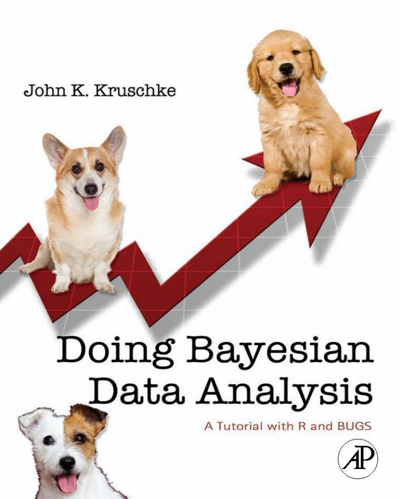
Doing Bayesian Data Analysis: A Tutorial with R and BUGS
Cover
Foreword
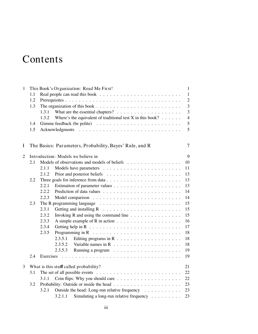
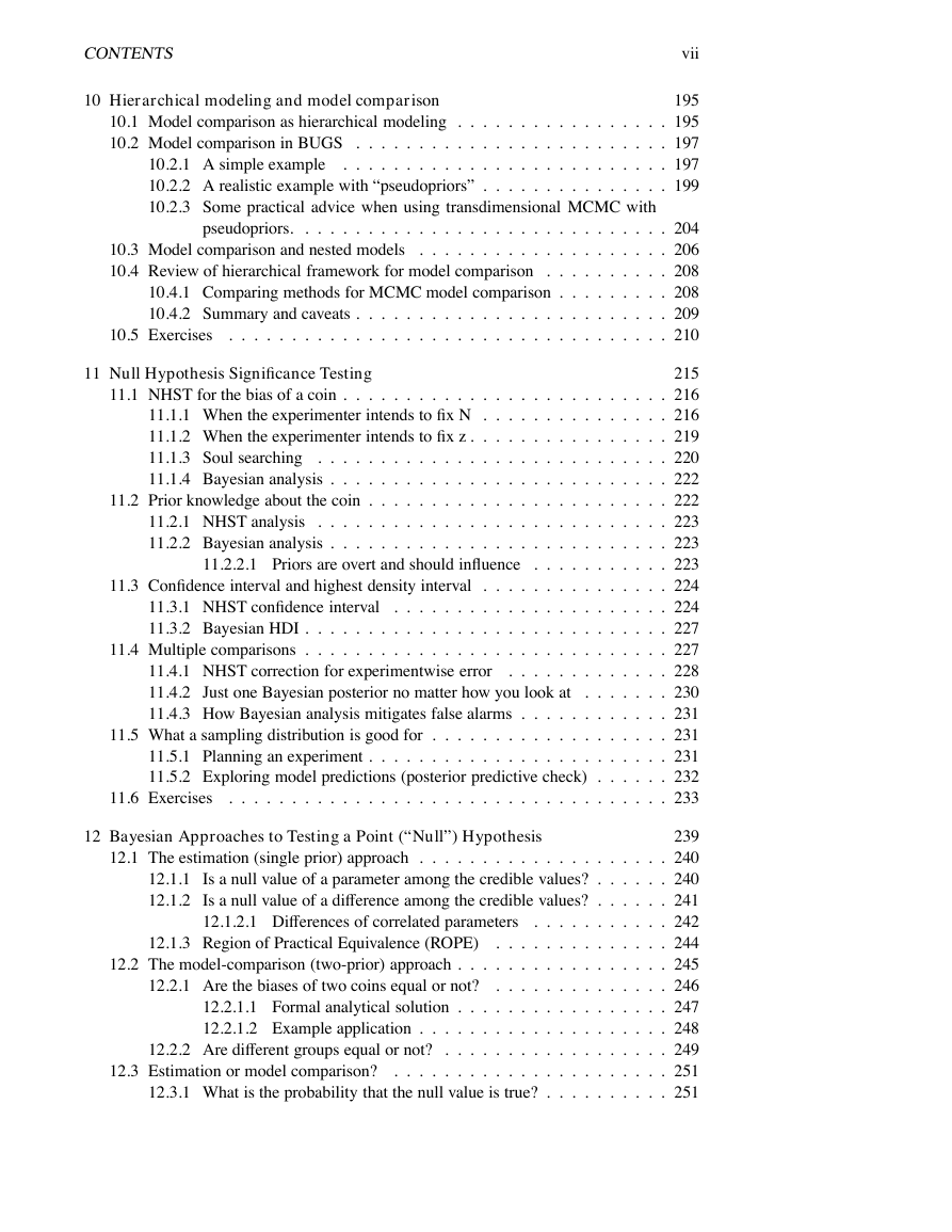
Contents
1 This Book’s Organization: Read Me First!
1.1 Real people can read this book
1.2 Prerequisites
1.3 The organization of this book
1.3.1 What are the essential chapters?
1.3.2 Where’s the equivalent of traditional test X in this book?
1.4 Gimme feedback (be polite)
1.5 Acknowledgments
I The Basics: Parameters, Probability, Bayes’ Rule, and R
2 Introduction: Models we believe in
2.1 Models of observations and models of beliefs
2.1.1 Models have parameters
2.1.2 Prior and posterior beliefs
2.2 Three goals for inference from data .
2.2.1 Estimation of parameter values
2.2.2 Prediction of data values
2.2.3 Model comparison
2.3 The R programming language
2.3.1 Getting and installing R
2.3.2 Invoking R and using the command line
2.3.3 A simple example of R in action
2.3.4 Getting help in R
2.3.5 Programming in R
2.3.5.1 Editing programs in R
2.3.5.2 Variable names in R
2.3.5.3 Running a program
2.4 Exercises
3 What is this stuff called probability?
3.1 The set of all possible events
3.1.1 Coin flips: Why you should care
3.2 Probability: Outside or inside the head
3.2.1 Outside the head: Long-run relative frequency
3.2.1.1 Simulating a long-run relative frequency
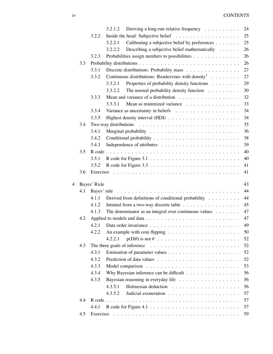
3.2.1.2 Deriving a long-run relative frequency
3.2.2 Inside the head: Subjective belief
3.2.2.1 Calibrating a subjective belief by preferences
3.2.2.2 Describing a subjective belief mathematically
3.2.3 Probabilities assign numbers to possibilities
3.3 Probability distributions
3.3.1 Discrete distributions: Probability mass
3.3.2 Continuous distributions: Rendezvous with density
3.3.2.1 Properties of probability density functions
3.3.2.2 The normal probability density function
3.3.3 Mean and variance of a distribution
3.3.3.1 Mean as minimized variance
3.3.4 Variance as uncertainty in beliefs
3.3.5 Highest density interval (HDI)
3.4 Two-way distributions
3.4.1 Marginal probability
3.4.2 Conditional probability
3.4.3 Independence of attributes
3.5 R code
3.5.1 R code for Figure 3.1
3.5.2 R code for Figure 3.3
3.6 Exercises
4 Bayes’ Rule
4.1 Bayes’ rule
4.1.1 Derived from definitions of conditional probability
4.1.2 Intuited from a two-way discrete table
4.1.3 The denominator as an integral over continuous values
4.2 Applied to models and data
4.2.1 Data order invariance
4.2.2 An example with coin flipping
4.2.2.1 p(D|θ) is not θ
4.3 The three goals of inference
4.3.1 Estimation of parameter values
4.3.2 Prediction of data values
4.3.3 Model comparison
4.3.4 Why Bayesian inference can be difficult
4.3.5 Bayesian reasoning in everyday life
4.3.5.1 Holmesian deduction
4.3.5.2 Judicial exoneration
4.4 R code
4.4.1 R code for Figure 4.1
4.5 Exercises
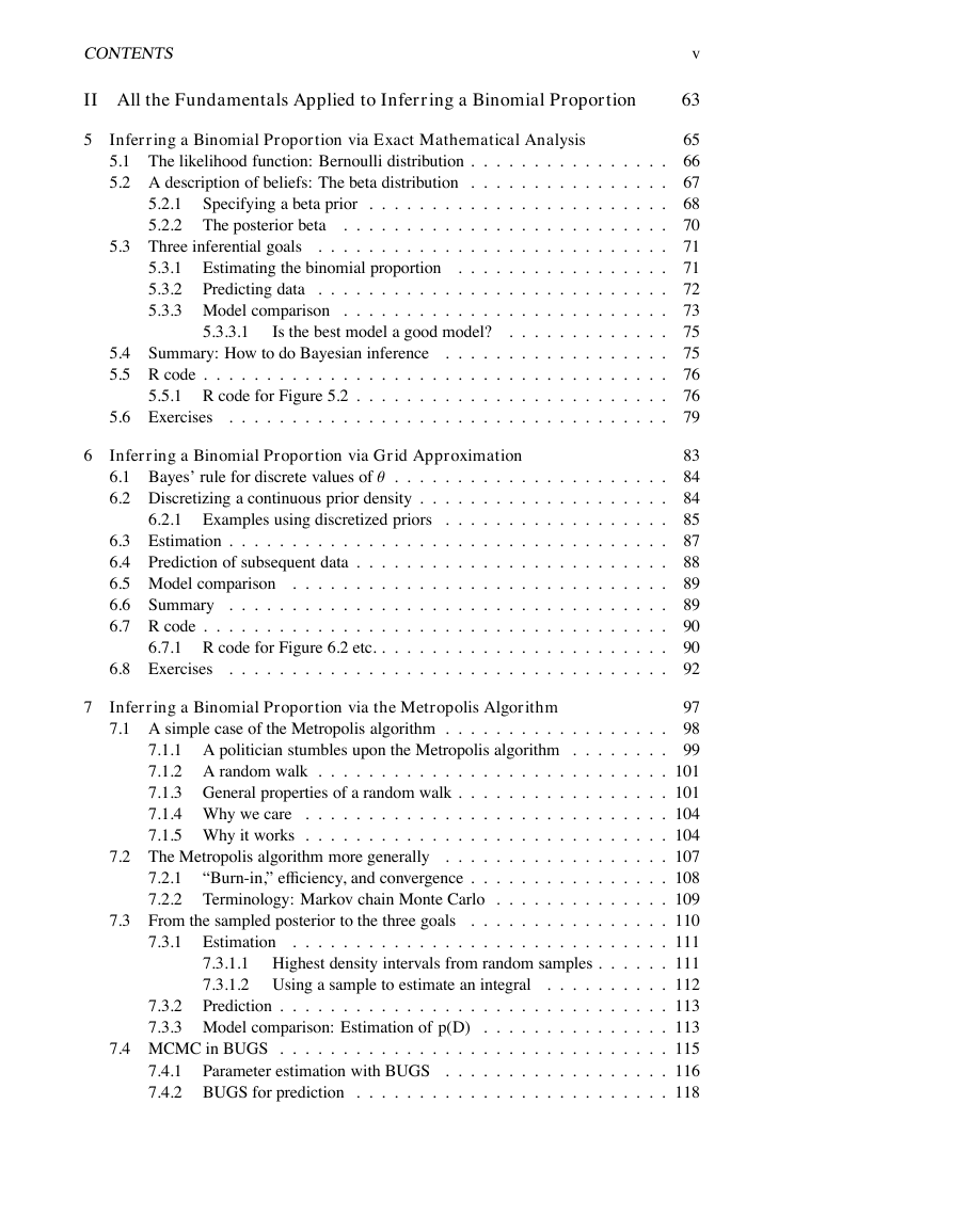
II All the Fundamentals Applied to Inferring a Binomial Proportion
5 Inferring a Binomial Proportion via Exact Mathematical Analysis
5.1 The likelihood function: Bernoulli distribution
5.2 A description of beliefs: The beta distribution
5.2.1 Specifying a beta prior
5.2.2 The posterior beta
5.3 Three inferential goals
5.3.1 Estimating the binomial proportion
5.3.2 Predicting data
5.3.3 Model comparison
5.3.3.1 Is the best model a good model?
5.4 Summary: How to do Bayesian inference
5.5 R code
5.5.1 R code for Figure 5.2
5.6 Exercises
6 Inferring a Binomial Proportion via Grid Approximation
6.1 Bayes’ rule for discrete values of θ
6.2 Discretizing a continuous prior density
6.2.1 Examples using discretized priors
6.3 Estimation
6.4 Prediction of subsequent data
6.5 Model comparison
6.6 Summary
6.7 R code
6.7.1 R code for Figure 6.2 etc
6.8 Exercises
7 Inferring a Binomial Proportion via the Metropolis Algorithm
7.1 A simple case of the Metropolis algorithm
7.1.1 A politician stumbles upon the Metropolis algorithm
7.1.2 A random walk
7.1.3 General properties of a random walk
7.1.4 Why we care
7.1.5 Why it works
7.2 The Metropolis algorithm more generally
7.2.1 “Burn-in,” efficiency, and convergence
7.2.2 Terminology: Markov chain Monte Carlo
7.3 From the sampled posterior to the three goals
7.3.1 Estimation
7.3.1.1 Highest density intervals from random samples
7.3.1.2 Using a sample to estimate an integral
7.3.2 Prediction
7.3.3 Model comparison: Estimation of p(D)
7.4 MCMC in BUGS
7.4.1 Parameter estimation with BUGS
7.4.2 BUGS for prediction
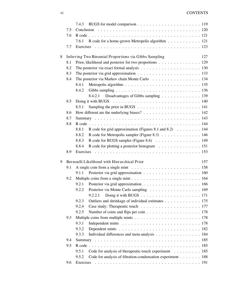
7.4.3 BUGS for model comparison
7.5 Conclusion
7.6 R code
7.6.1 R code for a home-grown Metropolis
7.7 Exercises
8 Inferring Two Binomial Proportions via Gibbs Sampling
8.1 Prior, likelihood and posterior for two proportions
8.2 The posterior via exact formal analysis
8.3 The posterior via grid approximation
8.4 The posterior via Markov chain Monte Carlo
8.4.1 Metropolis algorithm
8.4.2 Gibbs sampling
8.4.2.1 Disadvantages of Gibbs sampling
8.5 Doing it with BUGS
8.5.1 Sampling the prior in BUGS
8.6 How different are the underlying biases?
8.7 Summary
8.8 R code
8.8.1 R code for grid approximation (Figures 8.1 and 8.2)
8.8.2 R code for Metropolis sampler (Figure 8.3)
8.8.3 R code for BUGS sampler (Figure 8.6)
8.8.4 R code for plotting a posterior histogram
8.9 Exercises
9 Bernoulli Likelihood with Hierarchical Prior
9.1 A single coin from a single mint
9.1.1 Posterior via grid approximation
9.2 Multiple coins from a single mint
9.2.1 Posterior via grid approximation
9.2.2 Posterior via Monte Carlo sampling
9.2.2.1 Doing it with BUGS
9.2.3 Outliers and shrinkage of individual estimates
9.2.4 Case study: Therapeutic touch
9.2.5 Number of coins and flips per coin
9.3 Multiple coins from multiple mints
9.3.1 Independent mints
9.3.2 Dependent mints
9.3.3 Individual differences and meta-analysis
9.4 Summary
9.5 R code
9.5.1 Code for analysis of therapeutic-touch experiment
9.5.2 Code for analysis of filtration-condensation experiment
9.6 Exercises
10 Hierarchical modeling and model comparison
10.1 Model comparison as hierarchical modeling
10.2 Model comparison in BUGS
10.2.1 A simple example
10.2.2 A realistic example with “pseudopriors”
10.2.3 Some practical advice when using transdimensional MCMC withpseudopriors
10.3 Model comparison and nested models
10.4 Review of hierarchical framework for model comparison
10.4.1 Comparing methods for MCMC model comparison
10.4.2 Summary and caveats
10.5 Exercises
11 Null Hypothesis Significance Testing
11.1 NHST for the bias of a coin
11.1.1 When the experimenter intends to fix N
11.1.2 When the experimenter intends to fix z
11.1.3 Soul searching
11.1.4 Bayesian analysis
11.2 Prior knowledge about the coin
11.2.1 NHST analysis
11.2.2 Bayesian analysis
11.2.2.1 Priors are overt and should influence
11.3 Confidence interval and highest density interval
11.3.1 NHST confidence interval
11.3.2 Bayesian HDI
11.4 Multiple comparisons
11.4.1 NHST correction for experimentwise error
11.4.2 Just one Bayesian posterior no matter how you look at
11.4.3 How Bayesian analysis mitigates false alarms
11.5 What a sampling distribution is good for
11.5.1 Planning an experiment
11.5.2 Exploring model predictions (posterior predictive check)
11.6 Exercises
12 Bayesian Approaches to Testing a Point (“Null”) Hypothesis
12.1 The estimation (single prior) approach
12.1.1 Is a null value of a parameter among the credible values?
12.1.2 Is a null value of a difference among the credible values?
12.1.2.1 Differences of correlated parameters
12.1.3 Region of Practical Equivalence (ROPE)
12.2 The model-comparison (two-prior) approach
12.2.1 Are the biases of two coins equal or not?
12.2.1.1 Formal analytical solution
12.2.1.2 Example application
12.2.2 Are different groups equal or not?
12.3 Estimation or model comparison?
12.3.1 What is the probability that the null value is true?
12.3.2 Recommendations
12.4 R code
12.4.1 R code for Figure 12.5
12.5 Exercises
13 Goals, Power, and Sample Size
13.1 The Will to Power
13.1.1 Goals and Obstacles
13.1.2 Power
13.1.3 Sample Size
13.1.4 Other Expressions of Goals
13.2 Sample size for a single coin
13.2.1 When the goal is to exclude a null value
13.2.2 When the goal is precision
13.3 Sample size for multiple mints
13.4 Power: prospective, retrospective, and replication
13.4.1 Power analysis requires verisimilitude of simulated data
13.5 The importance of planning
13.6 R code
13.6.1 Sample size for a single coin
13.6.2 Power and sample size for multiple mints
13.7 Exercises
III The Generalized Linear Model
14 Overview of the Generalized Linear Model
14.1 The generalized linear model (GLM)
14.1.1 Predictor and predicted variables
14.1.2 Scale types: metric, ordinal, nominal
14.1.3 Linear function of a single metric predictor
14.1.3.1 Reparameterization to x threshold form
14.1.4 Additive combination of metric predictors
14.1.4.1 Reparameterization to x threshold form
14.1.5 Nonadditive interaction of metric predictors
14.1.6 Nominal predictors
14.1.6.1 Linear model for a single nominal predictor
14.1.6.2 Additive combination of nominal predictors
14.1.6.3 Nonadditive interaction of nominal predictors
14.1.7 Linking combined predictors to the predicted
14.1.7.1 The sigmoid (a.k.a. logistic) function
14.1.7.2 The cumulative normal (a.k.a. Phi) function
14.1.8 Probabilistic prediction
14.1.9 Formal expression of the GLM
14.2 Cases of the GLM
14.2.1 Two or more nominal variables predicting frequency
14.3 Exercises
15 Metric Predicted Variable on a Single Group
15.1 Estimating the mean and precision of a normal likelihood
15.1.1 Solution by mathematical analysis
15.1.2 Approximation by MCMC in BUGS
15.1.3 Outliers and robust estimation: The t distribution
15.1.4 When the data are non-normal: Transformations
15.2 Repeated measures and individual differences
15.2.1 Hierarchical model
15.2.2 Implementation in BUGS
15.3 Summary
15.4 R code
15.4.1 Estimating the mean and precision of a normal likelihood
15.4.2 Repeated measures: Normal across and normal within
15.5 Exercises
16 Metric Predicted Variable with One Metric Predictor
16.1 Simple linear regression
16.1.1 The hierarchical model and BUGS code
16.1.1.1 Standardizing the data for MCMC sampling
16.1.1.2 Initializing the chains
16.1.2 The posterior: How big is the slope?
16.1.3 Posterior prediction
16.2 Outliers and robust regression
16.3 Simple linear regression with repeated measures
16.4 Summary
16.5 R code
16.5.1 Data generator for height and weight
16.5.2 BRugs: Robust linear regression
16.5.3 BRugs: Simple linear regression with repeated measures
16.6 Exercises
17 Metric Predicted Variable with Multiple Metric Predictors
17.1 Multiple linear regression
17.1.1 The perils of correlated predictors
17.1.2 The model and BUGS program
17.1.2.1 MCMC efficiency: Standardizing and initializing
17.1.3 The posterior: How big are the slopes?
17.1.4 Posterior prediction
17.2 Hyperpriors and shrinkage of regression coefficients
17.2.1 Informative priors, sparse data, and correlated predictors
17.3 Multiplicative interaction of metric predictors
17.3.1 The hierarchical model and BUGS code
17.3.1.1 Standardizing the data and initializing the chains
17.3.2 Interpreting the posterior
17.4 Which predictors should be included?
17.5 R code
17.5.1 Multiple linear regression
17.5.2 Multiple linear regression with hyperprior on coefficients
17.6 Exercises
18 Metric Predicted Variable with One Nominal Predictor
18.1 Bayesian oneway ANOVA
18.1.1 The hierarchical prior
18.1.1.1 Homogeneity of variance
18.1.2 Doing it with R and BUGS
18.1.3 A worked example
18.1.3.1 Contrasts and complex comparisons
18.1.3.2 Is there a difference?
18.2 Multiple comparisons
18.3 Two group Bayesian ANOVA and the NHST t test
18.4 R code
18.4.1 Bayesian oneway ANOVA
18.5 Exercises
19 Metric Predicted Variable with Multiple Nominal Predictors
19.1 Bayesian multi-factor ANOVA
19.1.1 Interaction of nominal predictors
19.1.2 The hierarchical prior
19.1.3 An example in R and BUGS
19.1.4 Interpreting the posterior
19.1.4.1 Metric predictors and ANCOVA
19.1.4.2 Interaction contrasts
19.1.5 Non-crossover interactions, rescaling, and homogeneous variances
19.2 Repeated measures, a.k.a. within-subject designs
19.2.1 Why use a within-subject design? And why not?
19.3 R code
19.3.1 Bayesian two-factor ANOVA
19.4 Exercises
20 Dichotomous Predicted Variable
20.1 Logistic regression
20.1.1 The model
20.1.2 Doing it in R and BUGS
20.1.3 Interpreting the posterior
20.1.4 Perils of correlated predictors
20.1.5 When there are few 1’s in the data
20.1.6 Hyperprior across regression coefficients
20.2 Interaction of predictors in logistic regression
20.3 Logistic ANOVA
20.3.1 Within-subject designs
20.4 Summary
20.5 R code
20.5.1 Logistic regression code
20.5.2 Logistic ANOVA code
20.6 Exercises
21 Ordinal Predicted Variable
21.1 Ordinal probit regression
21.1.1 What the data look like
21.1.2 The mapping from metric x to ordinal y
21.1.3 The parameters and their priors
21.1.4 Standardizing for MCMC efficiency
21.1.5 Posterior prediction
21.2 Some examples
21.2.1 Why are some thresholds outside the data?
21.3 Interaction
21.4 Relation to linear and logistic regression
21.5 R code
21.6 Exercises
22 Contingency Table Analysis
22.1 Poisson exponential ANOVA
22.1.1 What the data look like
22.1.2 The exponential link function
22.1.3 The Poisson likelihood
22.1.4 The parameters and the hierarchical prior
22.2 Examples
22.2.1 Credible intervals on cell probabilities
22.3 Log linear models for contingency tables
22.4 R code for Poisson exponential model
22.5 Exercises
23 Tools in the Trunk
23.1 Reporting a Bayesian analysis
23.1.1 Essential points
23.1.2 Optional points
23.1.3 Helpful points
23.2 MCMC burn-in and thinning
23.3 Functions for approximating highest density intervals
23.3.1 R code for computing HDI of a grid approximation
23.3.2 R code for computing HDI of a MCMC sample
23.3.3 R code for computing HDI of a function
23.4 Reparameterization of probability distributions
23.4.1 Examples
23.4.2 Reparameterization of two parameters
References
Index
ii Dedicated to my mother, Marilyn A. Kruschke, and to the memory of my father, Earl R. Kruschke, who both brilliantly exemplified and taught sound reasoning. And, in honor of my father, who dedicated his first book to his children, I also dedicate this book to mine: Claire A. Kruschke and Loren D. Kruschke
Contents 1 This Book’s Organization: Read Me First! 1.1 Real people can read this book . . . . . 1.2 Prerequisites . . . . . . . . . . 1.3 The organization of this book . . . . . . . . . . . . . . . . . . . . . . . . . . . . . . . . . . . . . . . 1.3.1 What are the essential chapters? . . . . . . . . . . . 1.3.2 Where’s the equivalent of traditional test X in this book? . . . . . . . . . . . . . . . . 1.4 Gimme feedback (be polite) 1.5 Acknowledgments . . . . . . . . . . . . . . . . . . . . . . . . . . . . . . . . . . . . . . . . . . . . . . . . . . . . . . . . . . . . . . . . . . . . I The Basics: Parameters, Probability, Bayes’ Rule, and R 2 Introduction: Models we believe in Prior and posterior beliefs 2.1.1 Models have parameters 2.1.2 2.1 Models of observations and models of beliefs . . . . . . . . . . . . . . . . . . . . . . . . 2.2 Three goals for inference from data . . . . . . . . 2.2.1 Estimation of parameter values . . . . . . Prediction of data values . . . . 2.2.2 . . . . . . . . . . . 2.2.3 Model comparison . . . . . . 2.3 The R programming language . . . . . . . . . . 2.3.1 Getting and installing R . . . . 2.3.2 Invoking R and using the command line . 2.3.3 A simple example of R in action . . . . . . . . . . 2.3.4 Getting help in R . . Programming in R . 2.3.5 . . . . . Editing programs in R . . . . . 2.3.5.1 2.3.5.2 Variable names in R . . . . . . . . . . . Running a program . 2.3.5.3 . . . . . . . . . . . . . . . . . . . . . . . 2.4 Exercises . . . . . . . . . . . . . . . . . . . . . . . . . . . . . . . . . . . . . . . . . . . . . . . . . . . . . . . . . . . . . . . . . . . . . . . . . . . . . . . . . . . . . . . . . . . . . . . . . . . . . . . . . . . . . . . . 3 What is this stuff called probability? 3.1 The set of all possible events . . . . . . 3.2 Probability: Outside or inside the head . . . . . . 3.1.1 Coin flips: Why you should care . . . . . . . . . . . . . . . . . . . . . . . . . . . . 3.2.1 Outside the head: Long-run relative frequency . . . Simulating a long-run relative frequency . 3.2.1.1 iii . . . . . . . . . . . . . . . . . . . . . . . . . . . . . . . . . . . . . . . . . . . . . . . . . . . . . . . . . . . . . . . . . . . . . . . . . . . . . . . . . . . . . . . . . . . . . . . . . . . . . . . . . . . . . . . . . . . . . . . . . . . . . . . . . . . . 1 1 2 3 3 4 5 5 7 9 10 11 13 13 13 14 14 15 15 15 16 17 18 18 18 19 19 21 22 22 23 23 23 . . . . . . . . . . . . . . . . . . . . . . . . . . . . . . . . . . . . . . . . . . . . . . . . . . . . . . . . . .
iv CONTENTS 3.3 Probability distributions . . . 3.2.3 3.2.2 . . . . . . . . . . 3.3.2.1 3.3.2.2 . . . . . . 3.2.1.2 Deriving a long-run relative frequency . . . . . . . . Inside the head: Subjective belief . . . . . . 3.2.2.1 Calibrating a subjective belief by preferences . . . . . 3.2.2.2 Describing a subjective belief mathematically . . . . Probabilities assign numbers to possibilities . . . . . . . . . . . . . . . . . . . . . . . . . . . . . . . . . . 3.3.1 Discrete distributions: Probability mass . . . . . . . 3.3.2 Continuous distributions: Rendezvous with density† . . . . . . . . . . . . Properties of probability density functions . . . . . . The normal probability density function . . . . . . . . . . . . . . . . . . . . . . . . . . . . . . . . . . . . . . . . . . . . . . . . . . . . . . . . . . . . . . . . . . . . . . . . . . . . . . . . . . . . . . . . . . . . . . . . . . . . . . . . . . . . . . . . . . . . . . . . . . . . . . . . . . . . . . . . . . . . . . . . . 3.3.3 Mean and variance of a distribution . . . . . . . . . . . . . . . . . . . . . . . . . . . . . . . . . . . . . . . . . . . . . . . . . . . . . 3.3.4 Variance as uncertainty in beliefs 3.3.5 Highest density interval (HDI) . . . . . . . 3.4.1 Marginal probability . . . . . . 3.4.2 Conditional probability . . . . . 3.4.3 Independence of attributes . . . . . . . . . 3.5.1 R code for Figure 3.1 . . . . . . 3.5.2 R code for Figure 3.3 . . . . . . . . . . . . 3.3.3.1 Mean as minimized variance . . . . . . . . . . . . . . . . . . . . . 3.5 R code . 3.6 Exercises 3.4 Two-way distributions . . . 4 Bayes’ Rule 4.1 Bayes’ rule . . . . 4.3 The three goals of inference 4.2 Applied to models and data . 4.2.2.1 . . . . . . . . . . . . . . . . Intuited from a two-way discrete table . . . . . . . . . . . . . . . . . . . . 4.1.1 Derived from definitions of conditional probability . 4.1.2 . . . . . . . . . . . . 4.1.3 The denominator as an integral over continuous values . . . . . . . . . . . . . . . . . . . . . . . . . . . . . . . . . . . . . . . . . . . . . . . . . . . . . . . . . . . . . . . . . . . . . . . . . . . . . . . . . . . . . . . . . . . . . . . . . . . . . . . . . . . . . . . 4.2.1 Data order invariance . . . . . . . . . . . 4.2.2 An example with coin flipping . . . . . . p(D|θ) is not θ . . . . . . . . . . . . . . . . . . . . 4.3.1 Estimation of parameter values . . . . . . 4.3.2 Prediction of data values . . . . 4.3.3 Model comparison . . . . . . . . . . . . 4.3.4 Why Bayesian inference can be difficult . 4.3.5 Bayesian reasoning in everyday life . . . 4.3.5.1 Holmesian deduction . . . . . . . . . . 4.3.5.2 . . . . . . . . . . . . . . . Judicial exoneration . . . . . . . 4.4.1 R code for Figure 4.1 . . . . . . . . . . . . . . . . . . . . . . . . . . . . . . . . . . . . . . . . . . . . . . . . . . . . . . . . . . . . . . . . . . . . . . . . . . . . . . . . . . . . . . . . . . . . . . . . . . . . . . . . . . . . . . . . . . . . . . . . . . . 4.4 R code . 4.5 Exercises . . . . . . . . . . . . . . . . . . . . . . . . . . . . . . . . . . . . . . . . . . . . . . . . . . . . . . . . . . . . . . . . . . . . . . . . . . . . . . . . . . 24 25 25 26 26 26 27 27 29 30 32 33 34 34 35 36 38 39 40 40 41 41 43 44 44 45 47 47 49 50 52 52 52 52 53 56 56 56 57 57 57 59
CONTENTS II All the Fundamentals Applied to Inferring a Binomial Proportion 5 Inferring a Binomial Proportion via Exact Mathematical Analysis . . . . 5.3 Three inferential goals 5.2.1 5.2.2 The posterior beta Specifying a beta prior . . . . . . . . . . . . . . . . . 5.1 The likelihood function: Bernoulli distribution . . 5.2 A description of beliefs: The beta distribution . . . . . . . . . . . . . . . . . 5.3.1 Estimating the binomial proportion . . . 5.3.2 . . . . . Predicting data . . . . . . . . 5.3.3 Model comparison . Is the best model a good model? . . . . . . . . . . . . . . . . . . . 5.4 Summary: How to do Bayesian inference . . . . . . 5.5 R code . 5.5.1 R code for Figure 5.2 . . . . . . . . . . . . . . . . . . . . . . . . 5.6 Exercises . . . . . . . . . . . . . . . . . . . . . 5.3.3.1 . . . . . . . . . . . . . . . . . . . . . . . . . . . . . . . . . . . . . . . . . . . . . . . . . . . . . . . . . . . . . . . . . . . . . . . . . . . . . . . . . . . . . . . . . . . . . . . . . . . . . . . . . . . . . . . . . . . . . . . . . . . . . . . . . . . . . . . . . . . . . . . . . . . . . . . . . . . 6 Inferring a Binomial Proportion via Grid Approximation . . . . . 6.1 Bayes’ rule for discrete values of θ . . . 6.2 Discretizing a continuous prior density . . . . . . . . . . . 6.2.1 Examples using discretized priors . . . . . . . . . . . . . . . . . . . . . . . . . . . . . . . . . . . . . . . 6.3 Estimation . . . . . . . . . . . 6.4 Prediction of subsequent data . . . . . . 6.5 Model comparison . . . . . . . . . . . . . . . . . . . . . . 6.6 Summary . . . . . 6.7 R code . . . . . . . . . . . . . . . . . . 6.7.1 R code for Figure 6.2 etc. . . . . . . . . . . 6.8 Exercises . . . . . . . . . . . . . . . . . . . . . . . . . . . . . . . . . . . . . . . . . . . . . . . . . . . . . . . . . . . . . . . . . . . . . . . . . . . . . . . . . . . . . . . . . . . . . . . . . . . . . . . . . . . . . . . . . . . . . . . . . . . . . . . . . . 7 Inferring a Binomial Proportion via the Metropolis Algorithm . . . . . . 7.1 A simple case of the Metropolis algorithm . . . . . . . . . . . . . . . . . . . . . . . . . . . . . . . . . . . . . . . . . . . . . . . . . . . . 7.2.1 . . . . . . 7.2.2 Terminology: Markov chain Monte Carlo . . . . . . . . . . . . . . . . . . . . . . . . 7.1.1 A politician stumbles upon the Metropolis algorithm . . . . . . . . . . . . 7.1.2 A random walk . . . . . . . . . . . . . . 7.1.3 General properties of a random walk . . . 7.1.4 Why we care . . . . . . . . . . . . . . . . . . . . . . . . . . 7.1.5 Why it works . . . . . . . . . . 7.2 The Metropolis algorithm more generally . . . . . . . . . . “Burn-in,” efficiency, and convergence . . . . . . . . . . . . . . . . . . . . 7.3.1.1 Highest density intervals from random samples . . . . 7.3.1.2 Using a sample to estimate an integral . . . . . . . . . . . . Prediction . . . . . . . . . . . . . . . . . . . . . . . . . . . . . . . . . . . . Parameter estimation with BUGS . . . . . . . . . 7.3.2 7.3.3 Model comparison: Estimation of p(D) 7.4.1 7.4.2 BUGS for prediction . . . . . . . . . . . . . . . . . . . . . . . . . . . . . . . . . . . . . . 7.3 From the sampled posterior to the three goals 7.3.1 Estimation . . . . . 7.4 MCMC in BUGS . . . . . . . . . . . . . . . . . . . . . . . . . . . . . . . . . . . . v 63 65 66 67 68 70 71 71 72 73 75 75 76 76 79 83 84 84 85 87 88 89 89 90 90 92 . . . . . . . . . . . . . . . . . . . . . . . . . . . . . . . . . . . . . . . . . . . . . . 97 . . 98 . . 99 . . 101 . . 101 . . 104 . . 104 . . 107 . . 108 . . 109 . . 110 . . 111 . . 111 . . 112 . . 113 . . 113 . . 115 . . 116 . . 118
vi 7.5 Conclusion . . . . . . . . . . 7.6 R code . 7.4.3 BUGS for model comparison . . . . . . . . . . . . . . . . . . . . . . . . . . . . . . . . 7.6.1 R code for a home-grown Metropolis algorithm . . . . . . . . . . . . . . . . . . . . . . . . . . . . . . . . . . 7.7 Exercises . . . . . . . . . . . . . . . . . . . . . 8 Inferring Two Binomial Proportions via Gibbs Sampling CONTENTS . . . . . . . . . . . . . . . . . . . . . . . . . . . . . . . . 119 . . 120 . . 121 . . 121 . . 123 127 . . 129 . . 130 . . 133 . . 134 . . 135 . . 136 . . 139 . . 140 . . 141 . . 142 . . 143 . . 144 . . 144 . . 146 . . 149 . . 151 . . 153 157 . . 158 . . 160 . . 164 . . 166 . . 169 . . 171 . . 175 . . 177 . . 178 . . 178 . . 178 . . 182 . . 184 . . 185 . . 185 . . 185 . . 188 . . 191 8.5 Doing it with BUGS . . . . 8.4.1 Metropolis algorithm . . . . . . . . . . . . 8.4.2 Gibbs sampling . . . 8.1 Prior, likelihood and posterior for two proportions . . . . . . . . . . . 8.2 The posterior via exact formal analysis . . . . . . . . . . . . . 8.3 The posterior via grid approximation . . . . . . . . . . . . . 8.4 The posterior via Markov chain Monte Carlo . . . . . . . . . . . . . . . . . . . . . . . . 8.4.2.1 Disadvantages of Gibbs sampling . . . . . . . . . . . . . . . . . . . . . . . . . . . . . . . . . . . 8.8.1 R code for grid approximation (Figures 8.1 and 8.2) . . . . . 8.8.2 R code for Metropolis sampler (Figure 8.3) 8.8.3 R code for BUGS sampler (Figure 8.6) . . . . . . . 8.8.4 R code for plotting a posterior histogram . . . . . . . . . . . . . . . . . . . . . . 8.6 How different are the underlying biases? . . . . . . . . . . 8.7 Summary . . . . . 8.8 R code . . . . . . . . . . . . . . . . . . Sampling the prior in BUGS . . . . . . . . . . . . . . . . . . . . . . . . 8.9 Exercises . . . . . . . . . . . . . . . . . . . . . 8.5.1 . . . . . . . . . . . . . . . . . . . . . . . . . . . . . . . . . . . . . . . . . . . . . . . . . . . . . . . . . . . . . . . . . . . . . . . . . . . . . . . . . . . . . . . . . . . . . . . . . . . . . . 9 Bernoulli Likelihood with Hierarchical Prior 9.1.1 . . . . 9.2.1 9.2.2 9.1 A single coin from a single mint 9.2 Multiple coins from a single mint . . . . . . . . . Posterior via grid approximation . . . . . . . . . . Posterior via grid approximation . . . . . Posterior via Monte Carlo sampling . . . 9.2.2.1 Doing it with BUGS . . . . . . . . . . . . . . . . . . . . . . . . . . . . . . . . . . . . . . . . . . 9.2.3 Outliers and shrinkage of individual estimates . . . . . . . . . . 9.2.4 Case study: Therapeutic touch . . . . . . . . . . . . 9.2.5 Number of coins and flips per coin . . . . . . . . . . . . . . . . . . . . . . . . . . . . . . . . . . . . . Individual differences and meta-analysis . . . . . . . . . . . . . . . . . . . . . . . . . . . . . . . . . . . . . . . . . . . . . . . . . . . . . . . . . . . . . . . . . . . . . . . . . . . . . . . . . . . . . . . . . . . . . . . . . . . . . . . . . . . . . . . . . . . . . . . . . . . . . . 9.5.1 Code for analysis of therapeutic-touch experiment 9.5.2 Code for analysis of filtration-condensation experiment . . . . . . . . . . . 9.3.1 . 9.3.2 Dependent mints . . 9.3.3 9.3 Multiple coins from multiple mints . . . . . . . . . . . . . . . 9.4 Summary . . . . . 9.5 R code . . . . . . . . . . . . . . . . . . . Independent mints . . . . . . . . . . 9.6 Exercises . . . . . . . . . . . . . . . . . . . . . . . . . . .
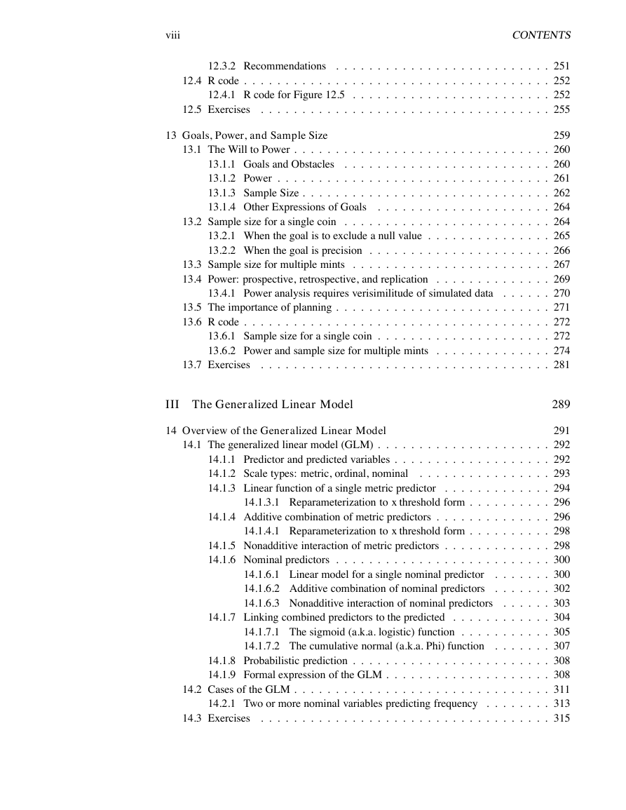
CONTENTS vii 10 Hierarchical modeling and model comparison 195 . . 195 . . 197 . . 197 . . 199 10.1 Model comparison as hierarchical modeling . . . . . . . . 10.2 Model comparison in BUGS . . . . . . 10.2.1 A simple example . . . . . . . . . . . 10.2.2 A realistic example with “pseudopriors” . 10.2.3 Some practical advice when using transdimensional MCMC with . . . . . . . . . . . . . . . . . . . . . . . . . . . . . . . . . . . . . . . . . . . . . . . . . . . . . pseudopriors. . . . . . . . . . . . . . 10.3 Model comparison and nested models . . . . . . 10.4 Review of hierarchical framework for model comparison . . 10.4.1 Comparing methods for MCMC model comparison . . . . . . . 10.4.2 Summary and caveats . . . . . . . . . . . . . . . . . . . . . . . . . . . . . . . . . . . . . . 10.5 Exercises . . . . . . . . . . . . . . . . . . . . . . . . . . . . . . . . . . . . . . . . . . . . . . 11 Null Hypothesis Significance Testing . . . . . . 11.1 NHST for the bias of a coin . 11.3 Confidence interval and highest density interval 11.2.1 NHST analysis . . . 11.2.2 Bayesian analysis . . . . . . . . . . . . . . 11.2 Prior knowledge about the coin . . . . . . . . . . . . . . . . . . . . . . 11.1.1 When the experimenter intends to fix N . 11.1.2 When the experimenter intends to fix z . . . . . . . 11.1.3 Soul searching . . . . . . . . 11.1.4 Bayesian analysis . . . . . . . . . . . . . . . . . . . . . . . . . . . . . . . . . . . . . . . . . . . . . . . . . . . . . . . . . . . . . . . . . 11.2.2.1 Priors are overt and should influence . . . . . . . . . . . . . . . . . . . . . . . . . . . . . . . . . . . . . . . . . . . 11.4.1 NHST correction for experimentwise error . . . . . 11.4.2 Just one Bayesian posterior no matter how you look at 11.4.3 How Bayesian analysis mitigates false alarms . . . . . . . . . . . . . . . . . . . . . . . . . . . . . . . . . . . . . . . . . . . . . . . . . . . . . . . . . . . . . . . . . . . . . . . . . . . . . . . . . . . . . . . . . . . . . . . . . . . . . . . . . . . . . . . . . . . . . 11.5.1 Planning an experiment . . . . . . . . . . . 11.5.2 Exploring model predictions (posterior predictive check) . . . . . . . . . . 11.3.1 NHST confidence interval 11.3.2 Bayesian HDI . . . . 11.4 Multiple comparisons . . . . 11.5 What a sampling distribution is good for . . . . . . . . . . . . . . . . . . . . . . . . . 11.6 Exercises . . . . . . . . . . . . . . . . . . . . . . . . . . . 12 Bayesian Approaches to Testing a Point (“Null”) Hypothesis . . . . . . . . . . . 12.1 The estimation (single prior) approach . 12.1.2.1 Differences of correlated parameters . . . . . . 12.1.1 Is a null value of a parameter among the credible values? . . . . 12.1.2 Is a null value of a difference among the credible values? . . . . . . . . . . . . . . . . . . . . . . . . . . . . . . . . . . . . . . . . . . . . . . . . . . . . . . . . . . . . . . . . . . . . . . . . . . . . . . . . . . . . . . . . . . . . . . . . . . . . . . . 12.3.1 What is the probability that the null value is true? . . 12.1.3 Region of Practical Equivalence (ROPE) 12.2 The model-comparison (two-prior) approach . . . 12.2.1 Are the biases of two coins equal or not? 12.2.1.1 Formal analytical solution . . . 12.2.1.2 Example application . . . . . . 12.2.2 Are different groups equal or not? . . . . . . . . . 12.3 Estimation or model comparison? . . . . . 204 . . 206 . . 208 . . 208 . . 209 . . 210 215 . . 216 . . 216 . . 219 . . 220 . . 222 . . 222 . . 223 . . 223 . . 223 . . 224 . . 224 . . 227 . . 227 . . 228 . . 230 . . 231 . . 231 . . 231 . . 232 . . 233 239 . . 240 . . 240 . . 241 . . 242 . . 244 . . 245 . . 246 . . 247 . . 248 . . 249 . . 251 . . 251
viii CONTENTS 12.4 R code . 12.3.2 Recommendations . . . . . . . . . . . . 12.4.1 R code for Figure 12.5 . . . . . . . . . . . . . . . . . . . . . . . . . . . . . . . . . . . . . . . . . . . . . . . . . . . . . . . . . . . . . . . . . . . . . . . . . . . . . . . . . . . . . . . . . . . . . . . . . . . . . . . 251 . . 252 . . 252 . . 255 12.5 Exercises 13 Goals, Power, and Sample Size 13.1 The Will to Power . . . . . . 13.1.1 Goals and Obstacles 13.1.2 Power . . . . . . . . 13.1.3 Sample Size . . . . . 13.1.4 Other Expressions of Goals . . . . . . . . . . . . . . . . . . . . . . . . . . 13.2 Sample size for a single coin . . . . . . . . . . . . . . . . . . . . . . . . . . . . . . . . . . . . . . . . . . . . . . . . . . . . . . . . . . . . . . . . . . . . . . . . . . . . . . 13.2.1 When the goal is to exclude a null value . . . . . . . . . . . . 13.2.2 When the goal is precision . . . 13.3 Sample size for multiple mints . . . . . . . . . . . . . . . . 13.4 Power: prospective, retrospective, and replication . . . . . . . . . . . . . . . . . . . . . . . . . . . . . . . . . . . . . . . . . . . . . . . . . . . . . . . . . . . . . . . . . . 13.4.1 Power analysis requires verisimilitude of simulated data . . . . . . . . . . . . . . . . . . . . . . . . . . . . . . . . . . . . . . . . . . . . . . . . . . . . . . . . . . . . . . . . 13.6.1 Sample size for a single coin . . 13.6.2 Power and sample size for multiple mints . . . . . . . . . . . . 13.5 The importance of planning . 13.6 R code . . . . . . . . . . . . . . . . . . . . . 13.7 Exercises . . . . . . . . . . . . . . . . . . . . . . . . . . . III The Generalized Linear Model 14 Overview of the Generalized Linear Model 14.1 The generalized linear model (GLM) . . . . . . . 14.1.1 Predictor and predicted variables . . . . . 14.1.2 Scale types: metric, ordinal, nominal . . 14.1.3 Linear function of a single metric predictor . . . . . . . . . . . . . . . . . . . . . . . 14.1.3.1 Reparameterization to x threshold form . . 14.1.4 Additive combination of metric predictors . . . . . . 14.1.4.1 Reparameterization to x threshold form . . 14.1.5 Nonadditive interaction of metric predictors . . . . . . . . . . . 14.1.6 Nominal predictors . 14.1.6.1 Linear model for a single nominal predictor 14.1.6.2 Additive combination of nominal predictors 14.1.6.3 Nonadditive interaction of nominal predictors . . . . . . . . . . . . . . . . . . . . . . . . . . . . . . . . . . . . . . . . . . . . . . . . . . . . . . . . . . . . . . . . . . . . . . . . . . 14.1.7 Linking combined predictors to the predicted . . . . 14.1.7.1 The sigmoid (a.k.a. logistic) function . . . . . . . . . 14.1.7.2 The cumulative normal (a.k.a. Phi) function . . . . . . . . . . . . . . . . . . . . . . . 14.2.1 Two or more nominal variables predicting frequency . . . . . . . . . . . . 14.1.8 Probabilistic prediction . . . . . 14.1.9 Formal expression of the GLM . . . . . . . . . . . . . . . . . . . . . . . . . . . . . . . . . . . . . . . . . . . . . . . . . . . . . . . . . . . . . . . . . . . . . . . . . . . . . . 14.2 Cases of the GLM . . . . . . 14.3 Exercises 259 . . 260 . . 260 . . 261 . . 262 . . 264 . . 264 . . 265 . . 266 . . 267 . . 269 . . 270 . . 271 . . 272 . . 272 . . 274 . . 281 289 291 . . 292 . . 292 . . 293 . . 294 . . 296 . . 296 . . 298 . . 298 . . 300 . . 300 . . 302 . . 303 . . 304 . . 305 . . 307 . . 308 . . 308 . . 311 . . 313 . . 315
分享到:
收藏