信息论与机器学习.pdf-资料库

96211087-b139-4543-9197-ffb893f6aed6.pdf-第1页.png

第1页 / 共49页

96211087-b139-4543-9197-ffb893f6aed6.pdf-第2页.png

第2页 / 共49页

96211087-b139-4543-9197-ffb893f6aed6.pdf-第3页.png

第3页 / 共49页

96211087-b139-4543-9197-ffb893f6aed6.pdf-第4页.png

第4页 / 共49页

96211087-b139-4543-9197-ffb893f6aed6.pdf-第5页.png

第5页 / 共49页

96211087-b139-4543-9197-ffb893f6aed6.pdf-第6页.png

第6页 / 共49页

96211087-b139-4543-9197-ffb893f6aed6.pdf-第7页.png

第7页 / 共49页

96211087-b139-4543-9197-ffb893f6aed6.pdf-第8页.png

第8页 / 共49页

Information Theory for Machine Learning Massimiliano Tomassoli (reverse(5102mnhuik)@gmail.com) 05/22/16 Contents 1 Introduction I The theory 2 Mean or Expected Value 3 Entropy 4 Entropy and Codes 4.1 Can we do better? . . . . . . . . . . . . . . . . . . . . . . . . . . 5 Logarithm and probabilities 6 Jensen’s Inequality 6.1 Convexity . . . . . . . . . . . . . . . . . . . . . . . . . . . . . . . 6.2 Deﬁnition and proof of Jensen’s Inequality . . . . . . . . . . . . . 7 Maximum Entropy 8 Specifying the distribution 9 Chain rule 10 Cross Entropy 11 Kullback-Leibler Divergence 12 Mutual Information 12.1 Deﬁnition . . . . . . . . . . . . . . . . . . . . . . . . . . . . . . . 12.2 Alternative formulation and interpretation . . . . . . . . . . . . . 12.3 Mutual Information VS Correlation . . . . . . . . . . . . . . . . . 12.4 Linear Regression . . . . . . . . . . . . . . . . . . . . . . . . . . . 1 2 3 3 9 9 11 12 14 14 15 17 19 19 20 21 22 22 24 24 25

13 A Set Theoretic view of Information Theory 13.1 The Inclusion Exclusion Principle . . . . . . . . . . . . . . . . . . 13.2 Cardinality of Intersections . . . . . . . . . . . . . . . . . . . . . 13.3 Multiple Mutual Information . . . . . . . . . . . . . . . . . . . . 13.4 KL Divergence and Total Correlation . . . . . . . . . . . . . . . . 26 27 30 31 37 II Applications of Information Theory to Machine Learn- ing 38 14 Loss function: from KL Divergence to Cross Entropy to Log Likelihood 14.1 Supervised Learning . . . . . . . . . . . . . . . . . . . . . . . . . 14.2 Density Estimation . . . . . . . . . . . . . . . . . . . . . . . . . . 15 Feature selection 15.1 Information Gain . . . . . . . . . . . . . . . . . . . . . . . . . . . 15.2 Joint Mutual Information . . . . . . . . . . . . . . . . . . . . . . 16 EM Algorithm 16.1 Bonus . . . . . . . . . . . . . . . . . . . . . . . . . . . . . . . . . 16.2 Deﬁnition . . . . . . . . . . . . . . . . . . . . . . . . . . . . . . . 16.3 Example . . . . . . . . . . . . . . . . . . . . . . . . . . . . . . . . 17 EM Algorithm: why does it work? 17.1 The MM Algorithm . . . . . . . . . . . . . . . . . . . . . . . . . 17.2 EM is an instance of MM . . . . . . . . . . . . . . . . . . . . . . 17.3 Information Theory interpretation . . . . . . . . . . . . . . . . . 38 38 39 40 41 41 42 42 42 43 45 45 46 48 Introduction 1 Students of Machine Learning are usually introduced to Information Theory through brief tutorials which are too superﬁcial to really understand what’s going on. One could always read a specialized book, but this might prove too much of an eﬀort for someone who doesn’t intend to become an expert in Information Theory. This tutorial wants to be a reasoned exposition where everything follows logically from what precedes it. I hope I succeeded in that. Because of the intended audience, some theorems are presented without proof but are thoroughly explained to give a solid intuition of why they’re true. 2

To make this tutorial self-contained, I took the liberty of proving some clas- sical results such as the Inclusion Exclusion Principle and Jensen’s Inequality as I needed them to prove other results. Moreover, I decided to conclude this tutorial with two sections about the celebrated EM Algorithm which I think everyone should know even if they’re just interested in, say, Deep Learning. I didn’t throw in the EM Algorithm just for the fun of it: there’s an interesting, if not strong, connection with Information Theory. A warning: every derivation is my own so keep your eyes open and let me know if you ﬁnd any mistakes! Part I The theory 2 Mean or Expected Value Before we dive into Information Theory, we’d better review the deﬁnition and some important properties of the mean or expected value. We’ll be focusing on the case of ﬁnite discrete random variables here, i.e. random variables which take only a ﬁnite number of values. For the inﬁnite case there are some subtleties about convergence. Also, for the continuous case one just have to replace all the sums with integrals. Deﬁnition 1. Let X be a discrete random variable with distribution p. The mean of X is deﬁned as EX∼p[X] = p(x)x. Remark 1. When there is no ambiguity, we can drop the distribution, the vari- able, or both: EX∼p[X] = EX [X] = Ep[X] = E[X]. x Deﬁnition 2. With a slight abuse of notation, if X is a random variable, we also see X as the set of values which X can take so that we can write, for instance, ∀x ∈ X, p(x) ∈ [0, 1]. Deﬁnition 3. If X is a random variable and f a function, then Z = f (X) is a random variable such that, for all z, p(z) = P (Z = z) = P (f (X) = z) = P (X ∈ f−1(z)) = p(x). x:f (x)=z Proposition 1. Let X be a random variable of distribution p and let f be a function. The mean of the random variable f (X) can be evaluated as follows Ef (X)[f (X)] = EX [f (X)] = p(x)f (x). x 3

Proof. Let Z = f (X) and let q be the distribution of Z. Then, Ef (X)[f (X)] = EZ[Z] z z x z z = = = = = q(z)z  x:f (x)=z x:f (x)=z  z p(x) p(x)z p(x)f (x) x:f (x)=z p(x)f (x) = EX [f (X)]. {x1, x2, . . . , xn} = Note that the double sum can be replaced with a single sum over x because z{x|f (x) = z}. ··· Deﬁnition 4. We can generalize deﬁnition 1 by considering a list of random variables X1, . . . , Xn: EX1,...Xn [f (X1, . . . , Xn)] = p(x1, . . . , xn)f (x1, . . . , xn). Deﬁnition 5. If X1, . . . , Xn are random variables, we can deﬁne a correspond- ing vector random variable as x1 xn X = (X1, . . . , Xn) = [X1 ··· Xn]t. Proposition 2. If X = (X1, . . . , Xn) and Y = (Y1, . . . , Ym) are vector random variables, i.e. vectors of random variables, then p(. . . , x, . . .) = p(. . . , x1, . . . , xn, . . .) p(. . . , x, . . .| . . . , y, . . .) = p(. . . , x1, . . . , xn, . . .| . . . , y1, . . . , ym, . . .), where x = (x1, . . . , xn) and y = (y1, . . . , yn). Proof. Let’s try not to be too technical. We’ll indicate events by writing predi- cates between curly braces. For instance, the event “X takes value x” is written as {X = x}. Now note that p(x, y) = p(X = x, Y = y) = P ({X = x} ∩ {Y = y}), which means that p(x, y) is really the probability of the intersection of the two events {X = x} and {Y = y}. Therefore, since X = x ⇐⇒ Xi = xi, i = 1, . . . , n, 4

then which means that {X = x} = {X1 = x1} ∩ ··· ∩ {Xn = xn}, p(. . . , x, . . .) = P (··· ∩ {X = x} ∩ ··· ) = P (··· ∩ {X1 = x1} ∩ ··· ∩ {Xn = xn} ∩ ··· ) = P (. . . , x1, . . . , xn, . . .). So, basically, a comma in these expressions means “and” or “intersection”. The proof for p(. . . , x, . . .| . . . , y, . . .) is analogous. Remark 2. Thanks to proposition 2, we can always simplify notation by writing just “X” or “x” instead of “X1, . . . , Xn” or “x1, . . . , xn”, respectively, and we can generalize results by doing the opposite. For instance, EX [f (X)] = p(x)f (x) ··· x implies the generalization EX1,...,Xn [f (X1, . . . , Xn)] = p(x1, . . . , xn)f (x1, . . . , xn). x1 xn Note that, to be precise, the f in the generalization is not exactly the same as the f in the simple case, but we won’t be afraid of abusing notation when convenient. Deﬁnition 6. The mean of a vector random variable X = (X1, . . . , Xn) is deﬁned as E[X] = (E[X1], . . . , E[Xn]). In general, if M is an m × n matrix random variable, then [E[M ]]ij = E[Mij] i = 1, . . . , m, j = 1, . . . , n. Proposition 3. The mean of a constant is equal to the constant itself. Proof. A constant c can be seen as a random variable X which takes the value c with probability 1. Thus, E[c] = EX [X] = p(x)x = c. Proposition 4. E[·] is linear. x 5

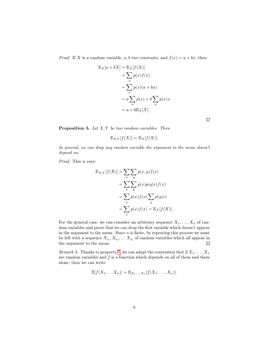
EX [a + bX] = EX [f (X)] x x = = p(x)f (x) p(x)(a + bx) Proof. If X is a random variable, a, b two constants, and f (x) = a + bx, then = a p(x) + b p(x)x x = a + bEX [X]. x Proposition 5. Let X, Y be two random variables. Then EX,Y [f (X)] = EX [f (X)]. In general, we can drop any random variable the argument to the mean doesn’t depend on. Proof. This is easy: EX,Y [f (X)] = = = = x x x y y p(x, y)f (x) p(x)p(y|x)f (x) p(x)f (x) p(y|x) y p(x)f (x) = EX [f (X)]. x For the general case, we can consider an arbitrary sequence X1, . . . , Xn of ran- dom variables and prove that we can drop the ﬁrst variable which doesn’t appear in the argument to the mean. Since n is ﬁnite, by repeating this process we must be left with a sequence Xi1, Xi2, . . . Xik of random variables which all appear in the argument to the mean. Remark 3. Thanks to property 5, we can adopt the convention that if X1, . . . , Xn are random variables and f is a function which depends on all of them and them alone, then we can write E[f (X1, . . . Xn)] = EX1,...,Xn [f (X1, . . . , Xn)]. 6

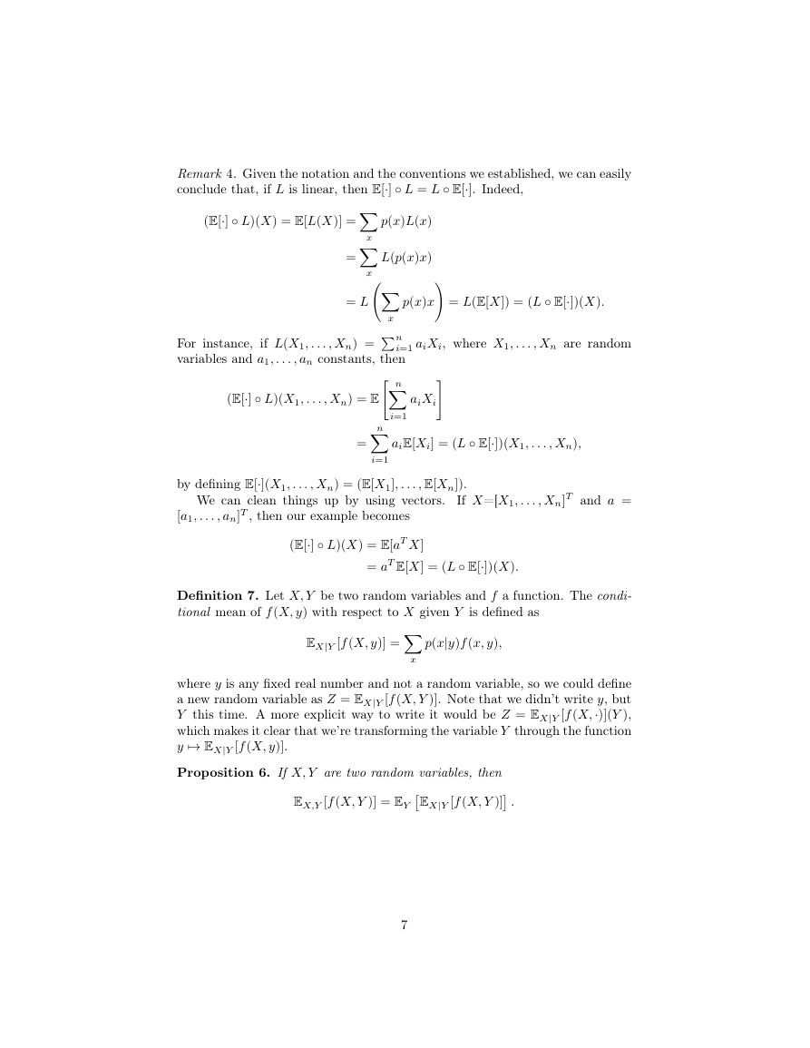
Remark 4. Given the notation and the conventions we established, we can easily conclude that, if L is linear, then E[·] ◦ L = L ◦ E[·]. Indeed, p(x)L(x) = L(p(x)x) x x (E[·] ◦ L)(X) = E[L(X)] = For instance, if L(X1, . . . , Xn) = n n n variables and a1, . . . , an constants, then (E[·] ◦ L)(X1, . . . , Xn) = E = L i=1 x aiXi = L(E[X]) = (L ◦ E[·])(X). p(x)x i=1 aiXi, where X1, . . . , Xn are random aiE[Xi] = (L ◦ E[·])(X1, . . . , Xn), = i=1 by deﬁning E[·](X1, . . . , Xn) = (E[X1], . . . , E[Xn]). We can clean things up by using vectors. [a1, . . . , an]T , then our example becomes If X=[X1, . . . , Xn]T and a = (E[·] ◦ L)(X) = E[aT X] = aT E[X] = (L ◦ E[·])(X). Deﬁnition 7. Let X, Y be two random variables and f a function. The condi- tional mean of f (X, y) with respect to X given Y is deﬁned as EX|Y [f (X, y)] = p(x|y)f (x, y), x where y is any ﬁxed real number and not a random variable, so we could deﬁne a new random variable as Z = EX|Y [f (X, Y )]. Note that we didn’t write y, but Y this time. A more explicit way to write it would be Z = EX|Y [f (X,·)](Y ), which makes it clear that we’re transforming the variable Y through the function y → EX|Y [f (X, y)]. Proposition 6. If X, Y are two random variables, then EX|Y [f (X, Y )] . EX,Y [f (X, Y )] = EY 7

Proof. The proof is easy: EX,Y [f (X, Y )] = = = x x y = EY y y p(x, y)f (x, y) p(x|y)p(y)f (x, y) EX|Y [f (X, Y )] . EX|Y,C[f (X, Y, c)] . p(x|y)f (x, y) p(y) x Proposition 7. If X, Y, C are random variables, then, for any ﬁxed c, EX,Y |C[f (X, Y, c)] = EY |C This is just a generalization of proposition 6. Proof. This proof can be derived from the proof of proposition 6 just by adding “|C”, “|c” and “, c” in the right places: EX,Y |C[f (X, Y, c)] = = = x x y p(x, y|c)f (x, y, c) EX|Y,C[f (X, Y, c)] . p(y|c) x y p(x|y, c)p(y|c)f (x, y, c) p(x|y, c)f (x, y, c) y = EY |C Corollary 1. If X, Y are independent random variables, then Proof. First of all, because X, Y are independent, in general, for any ﬁxed y, Now we can conclude the proof: EX,Y [XY ] = EY EX,Y [XY ] = EX [X]EY [Y ]. EX|Y [f (X, y)] = = p(x|y)f (x, y) p(x)f (x, y) x x 8 = EX [f (X, y)]. EX|Y [XY ] = EY [EX [XY ]] = EY [Y EX [X]] = EX [X]EY [Y ].

资料库

信息论与机器学习.pdf

相关推荐

课程资源

热门标签

最新资料