深度哈希方法综述（A Survey on Deep Hashing Methods）.pdf

发布时间：2022-05-31 发布人：admin 分类：说明书资料大小：0.38M 资料格式：pdf 举报版权申诉

syp_net-12237393-4744302542972776550.pdf-第1页.png

第1页 / 共23页

syp_net-12237393-4744302542972776550.pdf-第2页.png

第2页 / 共23页

syp_net-12237393-4744302542972776550.pdf-第3页.png

第3页 / 共23页

syp_net-12237393-4744302542972776550.pdf-第4页.png

第4页 / 共23页

syp_net-12237393-4744302542972776550.pdf-第5页.png

第5页 / 共23页

syp_net-12237393-4744302542972776550.pdf-第6页.png

第6页 / 共23页

syp_net-12237393-4744302542972776550.pdf-第7页.png

第7页 / 共23页

syp_net-12237393-4744302542972776550.pdf-第8页.png

第8页 / 共23页

1 Introduction

2 Background

3 Deep Supervised Hashing

4 PAIRWISE SIMILARITY PRESERVING

5 Multiwise similarity preserving

6 Implicit similarity preserving

7 Classification-oriented deep hashing

8 Quantization-based deep Hashing

9 Other Topic in Deep Supervised Hashing

10 Evaluation protocols

11 Conclusion

Noname manuscript No. (will be inserted by the editor) A Survey on Deep Hashing Methods Xiao Luo1,2 Minghua Deng1 · Jianqiang Huang2 · Xiansheng Hua2 · Chong Chen1,2∗ · Huasong Zhong2 · Hao Zhang2 · 0 2 0 2 r a M 4 ] V C . s c [ 1 v 9 6 3 3 0 . 3 0 0 2 : v i X r a Received: date / Accepted: date Abstract Nearest neighbor search is to ﬁnd the data points in the database such that the distances from them to the query are the smallest, which is a funda- mental problem in various domains, such as computer vision, recommendation systems and machine learning. Hashing is one of the most widely used method for its computational and storage eﬃciency. With the devel- opment of deep learning, deep hashing methods show more advantages than traditional methods. In this pa- per, we present a comprehensive survey of the deep hashing algorithms. Based on the loss function, we cat- egorize deep supervised hashing methods according to the manners of preserving the similarities into: pairwise similarity preserving, multiwise similarity preserving, implicit similarity preserving, as well as quantization. In addition, we also introduce some other topics such as deep unsupervised hashing and multi-modal deep hash- ing methods. Meanwhile, we also present some com- Xiao Luo E-mail: xiban.lx@alibaba-inc.com Chong Chen E-mail: cheung.cc@alibaba-inc.com Huasong Zhong E-mail: huasong.zhs@alibaba-inc.com Hao Zhang E-mail: puhong.zh@taobao.com Minghua Deng E-mail: dengmh@math.pku.edu.cn Jianqiang Huang E-mail: jianqiang.hjq@alibaba-inc.com Xiansheng Hua E-mail: xiansheng.hxs@alibaba-inc.com 1. School of Mathematical Sciences, Peking University 2. Damo Academy, Alibaba Group *. Corresponding author monly used public datasets and the scheme to measure the performance of deep hashing algorithms. Finally, we discussed some potential research directions in the conclusion. Keywords Approximate nearest neighbor search · learning to hashing · deep neural network · similarity preserving · deep supervised hashing 1 Introduction Nearest neighbor search is one of the most basic prob- lems in many ﬁelds, such as computer vision, recom- mendation systems, and machine learning. Its purpose is to ﬁnd the closest point from the dataset to the query based on a certain distance. However, when the amount of data is large and the dimensions are high, the time cost of accurately ﬁnding the point closest to the query is very large. To solve this problem, people began to pay more attention to approximate nearest neighbor search because in most cases it can meet the search needs and greatly reduce the search complexity. Hashing is one of the most widely used methods be- cause it is very eﬃcient in terms of computation and storage. Its purpose is to convert the original features of high latitudes into low-dimensional hash codes, so that the hash codes of the original similar objects are as close as possible, and the hash codes of dissimilar objects are as diﬀerent as possible. The existing hash- ing methods are mainly divided into two categories, one is local sensitive hashing [18,59], and the other is learning to hashing. The purpose of local sensitive hashing is to map the original data into several hash buckets, so that the closer the original distance objects are, the greater the probability that they will fall in the

2 Short form of author list same hash bucket. Through this mechanism, many al- gorithms based on locally sensitive hashing have been proposed [5,6,27,28,96,99], which show high superior- ity in both calculation and storage. However, in order to improve the recall rate of search, these methods usu- ally need to build many diﬀerent hash tables, so their application on particularly large data sets is still lim- ited. Since local sensitive hashing is data independent, people try to get high quality hashing codes by learn- ing good hash functions. Since the two early algorithms, semantic hashing [102,103] and spectral hashing [118] that learns projection vectors instead of the random projections, learning to hash has been attracting a large amount of research interest in computer vision and ma- chine learning. With the development of deep learning [75], getting hashing code through deep learning gets more and more attention for two reasons. The ﬁrst rea- son is that the powerful representation capabilities of deep learning can learn very complex hash functions. The second reason is that deep learning can achieve end-to-end hashing codes, which is very useful in many applications. In this survey, we mainly focus on deep supervised hashing methods and some other topics are also included. The design of the deep supervised hashing method mainly includes two parts, namely the design of the net- work structure and the design of the loss function. For small dataset like MINST [76] and CIFAR-10 [71], shal- low architecture such as AlexNet [73] and CNN-F [19] are widely used. While for complex dataset like NUS- WIDE [25] and COCO [86], deeper architecture such as VGG [107] and ResNet50 [50] are needed. The intu- ition of the loss function design is to maintain similarity, such as minimizing the gap between the similarity in the original space and the similarity in the hash space. The similarity in the original space is usually obtained by using semantic label information or the distance rela- tionship in the original space, which is widely studied in diﬀerent deep hashing methods. Hence we mainly focus on the similarity preserving manners latter. Following to [116], we also categorizes the deep hash- ing algorithms according to the similarity preserving manners into: pairwise similarity preserving, multiwise similarity preserving, implicit similarity preserving, quan- tization and classiﬁcation oriented. For each manner, We comprehensively analyzed how the related article designs the loss function, takes advantages of semantic labels and what additional tricks are used. In addition, we also introduce some other topics such as deep unsu- pervised hashing and multi-modal deep hashing meth- ods. Meanwhile, we also present some commonly used public datasets and the scheme to measure the perfor- mance of deep hashing algorithms. At last, a compari- son of some key algorithms was given. In comparison to other surveys on hash [115,114, 116,15], this survey mainly focuses on deep hashing methods and how they design loss functions. As far as we know, this is the most comprehensive survey about deep hashing, which is helpful for readers to understand the mechanisms and trends of deep hashing. 2 Background 2.1 Nearest neighbor search Given a d-dimensional Euclidean space Rd, the nearest neighbor search problem is to ﬁnd the element NN(x) in a ﬁnite set Y ⊂ Rd with n points such that NN(x) = argminy∈Y ρ(x, y), (1) where x ∈ RD is called a query. The distance ρ can be by Euclidean distance, general ℓp distance, cosine simi- larity and so on. Many exact nearest neighbor search method such as KD-tree [35] were developed by re- searcher, which works quite well when d is small. How- ever, Nearest neighbor search is inherently expensive due to the curse of dimensionality [2] [3]. Although KD- tree can be extended to high-dimensional situations, the eﬀect is not very good, even slower than brute force search. To solve this problem, a series of algorithms for ap- proximate nearest neighbors have been proposed [28, 40,97,62]. The principle of these methods is to ﬁnd the nearest point with a high probability, rather than to ﬁnd the nearest point accurately. These ANN algo- rithms are mainly divided into three categories: hashing- based [28,1,93], product quantization based [62,37,68, 132] and graph based [46,94,95]. These algorithms have greatly improved the eﬃciency of searching while ensur- ing a relatively high accuracy rate, so they are widely used in the industry. Compared to the other two types of methods, hash-based algorithms are the longest stud- ied and the most studied by people at the same time. Because it has great potential in improving computing eﬃciency and reducing memory cost. 2.2 Search with hashing The Purpose of the hash algorithm is to map the fea- tures of the original space into a Hamming space, which results in a short compact hashing code consists of 0 and 1. Because the computer’s calculations and storage are implemented in binary, hash coding is very eﬃcient in storage and calculation. There are two main types

A Survey on Deep Hashing Methods 3 of hash-based search algorithms: hash table lookup and hash code ranking. The main idea of hash table lookup for accelerat- ing the search is reducing the number of the distance computations. The data structure, called hash table (a form of inverted index), is composed of buckets with each bucket indexed by a hash code. Each point is as- signed to a hash bucket which shares the same hash code. Therefore, the strategy for learning hash encoding for this type of algorithm is to make the relatively close points in the original space have a higher probability of having the same hash encoding. When a query comes, we can ﬁnd the corresponding hash bucket according to the hash code of the query, so as to ﬁnd the correspond- ing candidate set. After this step, we usually re-rank the points in the candidate set to get the ﬁnal search target. However, the recall of selecting a single hash bucket as a candidate set will be relatively low. To overcome this problem, two methods are usually adopted. The ﬁrst method is to select some buckets that are close to the target bucket at the same time. The second method is to independently create multiple diﬀerent hash tables according to diﬀerent hash codes. Then we can select the corresponding target bucket from each hash table. Hash code ranking is a relatively easier way than hash table lookup. When a query comes, we simply compute the Hamming distance between query and each points in the searching dataset. Then select the points with relative smaller Hamming distance as the can- didates for nearest neighbor search. After that, a re- ranking process by the original features is usually fol- lowed to obtain the ﬁnal nearest neighbor. Diﬀer to hash table lookup methods, Hash code ranking methods prefer hash codes that preserve the similarity/distance of the original space. 2.3 Deep neural network Deep Convolutional Neural Networks (CNNs), a spe- cial type of Neural Networks, which have shown signif- icant performance improvement in several Image Pro- cessing and Computer Vision competitions, such as Im- ageNet [73]. The powerful and eﬀective learning ability of deep CNN is mainly derived from the utilization of multiple feature extraction stages that can automati- cally learn feature representations from the origin im- ages. In 2012, A. Krizhevsky et al. [73] drew atten- tion to the public by AlexNet network which achieved a top-5 error rate of 15.3% outperforming the previ- ous best traditional model in ImageNet dataset. Since the 2012 milestone, many researcher have tried to go deeper in the sequences of convolution layers to achieve better performance. In 2014, K. Simonyan & A. Zis- serman [108] introduced the 16-layers VGG model that chains multiple convolution layers to win this compe- tition. The same year, M. Lin et al. [85] have devel- oped the concept of inception modules which is further exploited by C. Szegedy et al. [112] who proposed a deeper network called GoogLeNet with 22 layers. The main common trend to design convolutional neural net- work models is the increasing network depth. However, as the depth increased, networks involved an increas- ing error rate due to the diﬃculties to optimize an ex- tremely deep models. K. He et al. [51] proposed ResNet network by residual learning to further deepen network to 101 layers. To avoid the tedious network architec- tures design, Google Brain researchers (B. Zoph and Q.V. Le, 2017) [138] have proposed a new concept called Neural Architecture Search(NAS) which searches state- of-the-art networks automatically. After that, various NAS networks have been released to the community, such as PNAS [88], ENAS [100], EﬃcientNet [113] and so on. And these classic network architectures further become the backbone networks in other tasks, such as image retrieval [116] and object detection [47]. 3 Deep Supervised Hashing 3.1 Learning to Hash Given an input item x, learning to hash is the task of learning a hash function f , which maps x to a compact hash code b for the convenience of the nearest neighbor search. The hash code obtained by a good hash func- tion should preserve the distance order in the original space as much as possible, i.e. those items that are close to query by hash code should also be close to query in the original space. Many traditional hash functions in- cluding linear projection, kernels, spherical function, a non-parametric function[116,110,48] were proposed by researchers to learn compact hash codes, and achieved signiﬁcant progress. However, these simple hash func- tion do not work well for large dataset. For the strong representation ability of deep learning, more and more researchers pay attention to deep supervised hashing and develop a lot of new methods. And these methods achieve higher performance than traditional methods. Deep supervised hashing uses deep neural networks as hash functions, which can generate hash code end- to-end. A good deep supervised hashing model usually needs to consider four issues: what deep neural net- work architecture is adopted, how to take advantage of the similarity and semantic(class) information, how to train the neural network with the discretization prob-

4 Short form of author list lem and what other skills can be used to improve the performance. 3.2 Network Architecture Traditional hashing methods usually utilize linear pro- jection and kernels, which shows poor representation ability. After AlexNet and VGGNet[73,107] were pro- posed, deep learning shows its superiority in computer vision, especially for classiﬁcation problems. And more and more experiments proved that the deeper the net- work, the better the performance. As a result, ResNet [50] takes advantage of residual learning, which can train very deep networks, achieved signiﬁcantly better results. After that, ResNet and its variants become ba- sic architectures in deep learning[50,55,121]. The latest researches often utilize the popular architectures with pre-trained weights in the large datasets such as Im- ageNet, following the idea of transfer learning. Most of researches utilize the shallower architectures such as AlexNet, CNN-F and designed stacked convolutional neural networks for simple datasets, e.g. MINST, CIFAR- 10. Deeper architectures such as VGGNet and ResNet50 are often utilized for complex datasets such as NUS- WIDE and COCO. For deep supervised hashing meth- ods, the last layer (i.e. classiﬁcation layer) is often re- placed by a hash layer, which has a dense connection with the feature layer. And the hash code can be ob- tained by the output of hash layer with a sign activa- tion. The network architecture is one of the most impor- tant factors for deep supervised hashing, and it aﬀects both the accuracy of the search and the time cost of in- ference. If the architecture is degenerated into MLP or linear projections, the deep supervised hashing become the traditional hashing methods. Although the deeper the network architecture, the greater the search accu- racy, but it also increases the time cost. We think that the architecture need to be considered combined with the complexity of datasets. However, all the deep hash- ing methods can change their architectures without any the other change. Therefore, we do not use the network architecture to categorize the deep supervised hashing algorithms. 3.3 Similarity In the rest, we always deﬁne xi as the input, hi as the output of the network, bi as the obtained binary codes, for each sample i. We denote the distance be- tween pair of items (xi, xj )in the input space and hash ij and sh coding space as so ij , respectively. In the in- put space the similarity is the ground truth, which mainly includes items distance do ij and semantic sim- ilarity. The former is the distance of features, e.g. Eu- clidean distance||xi − xj||2 and the similarity can be de- ﬁned by Gaussian function or Characteristic function, (do ij)2 2σ2 , Ido i.e. exp− ij <τ , in which τ is a given thresh- old. The cosine similarity is also popular. The similarity is usually binary in deep supervised hashing, where the value is 1 if the two items have common semantic label and 0 vice visa. In the hash coding space, the distance dh ij is Ham- ming distance naturally, which is deﬁned as the number of bits where the values are diﬀerent and is formulated as: dh ij = M Xm=1 δ [bim 6= bjm] , If the code is valued by 1 and 0, we have dh ij = kbi − bjk1 , and it varies from 0 to M. As a result, the similarity based on the Hamming distance is deﬁned as sh ij = M − dh ij. If the code is valued by 1 and -1, we have dh ij = 1 2 (M − bT i bj), ij = i bj. These measures can also be extended to the The similarity is deﬁned by the inner product, i.e.sh b⊤ weighted cases. i.e. dh ij = M Xm=1 λmδ [bim 6= bjm] , in which each bit has a weight λm, and if the codes are valued by 1 and -1, we have sh ij = b⊤ i Λbj ′ , where Λ = Diag (λ1, λ2, . . . , λM ) is a diagonal matrix and each diagonal entry is the weight of the correspond- ing hash bit. 3.4 Loss Function A good loss function is one of the factors for the suc- cess of deep supervised hashing. The basic rule of de- signing the loss function is to preserve the similarity order, i.e. minimizing the gap between the similarity in the original space and the similarity in the hash space. As a result, almost all the loss functions contain the

A Survey on Deep Hashing Methods 5 terms of similarity information. For example, the typ- ical loss function is pair-wise loss, making similar im- ages have similar hash codes (small hamming distance) and dissimilar images have dissimilar hash codes (large hamming distance). Besides, the multi-wise similarity preserving loss term, especially in triplet forms, mak- ing the orders among multiple items computed from the original and new spaces as consistent as possible, is also widely utilized. There are also several implicit and other variants similarity preserving loss terms. Besides similarity information, the semantic(label) information is also included for the design of loss func- tion. There are three popular ways to take advantage of label information that are summarized below. The ﬁrst way is regression on hash codes with label. The label is encoded into one-hot format matrix and regres- sion loss, i.e.||Y − W H||F are added into loss function. The second way is adding a classiﬁcation layer after the hash layer, and classiﬁcation loss(cross-entropy loss)are added to the loss function. The last one is utilizing Lab- Net, which was ﬁrst proposed in [79]. The principle of LabNet is explored to capture abundant semantic cor- relation between sample pairs. The quantization loss term is also common in deep supervised hashing, especially in quantization-based hash- ing methods. There are also several skills can be added in loss function, e.g. bit balancing, regularization, and so on, which is also important for improving the per- formance. 3.5 Optimization The challenges for optimizing the neural network pa- rameters is the vanishing gradient problem form sign function which is used to obtain binary hash codes. Speciﬁcally, the gradient of sign function is zero for all nonzero input, and that is fatal to the neural network which uses gradient descent for training. Almost all the works adopt that continuous relax- ation by replacing sign function with tanh or sigmoid, and later in test phase apply sign function to obtain ﬁnal binary codes. The ﬁrst typical way is quantiza- tion function by adding a penalty term in loss func- tion, which is often formulated as |||hi| − 1||1, or −||hi|| with tanh activation. This penalty term helps the neu- ral network to obtain sgn(z) ≈ z. It’s noticed that this loss can be considered as a novel prior for each hash code h based on a symmetric variant of some distribu- tion, e.g. bimodal Laplacian and Cauchy distribution. From this view we can get some variants, e.g. pairwise quantization[137] and Cauchy quantization loss[12]. If the loss function is non-smooth function whose deriva- tive is diﬃcult to compute, a smooth surrogate can be adopted, e.g. |x| ≈ log(cosh x), which helps get the smooth loss function[137]. The second way is an alter- native scheme, which decompose the optimization into several sub-problems, which can be iteratively solved by using the alternating minimization method. In this alternative process, back propagation can only works in one sub-problem and the other sub-problems can be solved by other optimization methods. For exam- ple, DSDH[80] utilizes the discrete cyclic coordinate de- scend algorithm. This methods can keep the discrete constraint during the whole optimization process while it can not lead to end-to-end training, which have lim- ited application for solving the unknown sub-problems. The third method is named continuation which utilizes a smooth activation function y = tanh(βx) to approx- imate the discrete sign function by increasing β [16]. There are some other ways to solve this problem by changing the calculation and the propagation of gra- dients, e.g. Greedy Hash[111] and Gradient Attention Network[56], which improved the eﬀectiveness and ac- curacy of deep supervised hashing. 3.6 Categorization Our survey categorizes the existing algorithms to the following ﬁve classes base on the similarity preserve manners: the pairwise similarity preserving class, the multi-wise similarity preserving class, the implicit sim- ilarity preserving class, the quantization class and clas- siﬁcation oriented class. We separate the quantization class from the pairwise similarity preserving class sim- ilar to [116]. For each class, we will discuss the corre- sponding deep hashing methods in detail one by one. 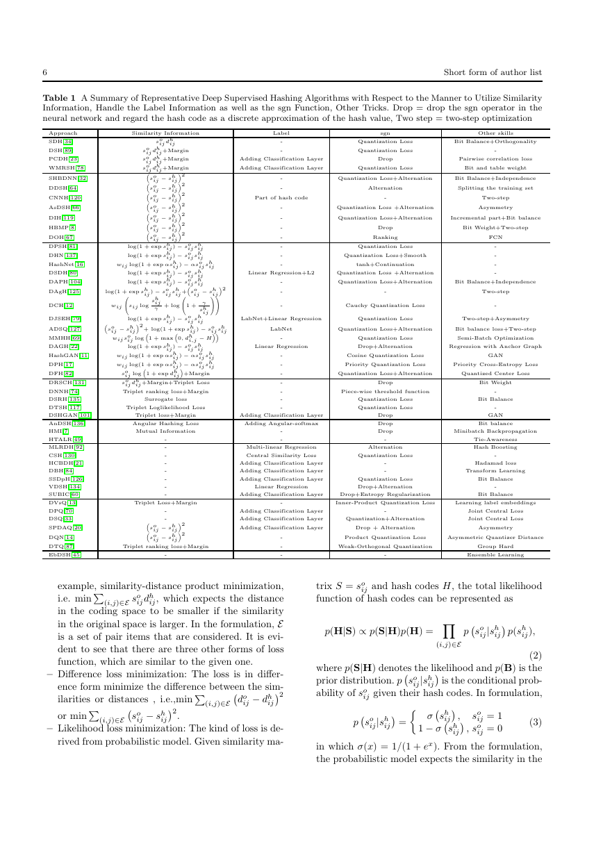The summary of these algorithms is shown in Table 1. The main reason we choose the similarity preserv- ing manner to do the categorization is that similarity preservation is the essential goal of hashing, which is al- most essential in loss function in deep supervised hash- ing. Other factors such as architecture, label informa- tion, optimization as well as other skills is also signiﬁ- cant for the performance. 4 PAIRWISE SIMILARITY PRESERVING The algorithms aligning the distances or similarities of a pair of items computed from the input space and the Hamming coding space are roughly divided into the fol- lowing groups: – Product loss minimization: The loss is in the prod- uct form of the similarity information between the input space and hash coding space. The similar- ity information includes distance and similarity. For

6 Short form of author list Table 1 A Summary of Representative Deep Supervised Hashing Algorithms with Respect to the Manner to Utilize Similarity Information, Handle the Label Information as well as the sgn Function, Other Tricks. Drop = drop the sgn operator in the neural network and regard the hash code as a discrete approximation of the hash value, Two step = two-step optimization Label - - sgn Other skills Quantization Loss Bit Balance+Orthogonality Quantization Loss - Adding Classification Layer Drop Pairwise correlation loss Adding Classification Layer Quantization Loss Bit and table weight - - Quantization Loss+Alternation Bit Balance+Independence Alternation Splitting the training set Part of hash code - Quantization Loss +Alternation Quantization Loss+Alternation Incremental part+Bit balance Drop Ranking Quantization Loss Quantization Loss+Smooth tanh+Continuation Two-step Asymmetry Bit Weight+Two-step FCN - - - - Linear Regression+L2 Quantization Loss +Alternation - - - Quantization Loss+Alternation Bit Balance+Independence - Two-step Cauchy Quantization Loss - LabNet+Linear Regression Quantization Loss Two-step+Asymmetry LabNet - Quantization Loss+Alternation Bit balance loss+Two-step Quantization Loss Semi-Batch Optimization Linear Regression Drop+Alternation Regression with Anchor Graph - - - - - - - - - - - - - - Similarity Information ij dh ij − sh so ij so dh ij +Margin ij so dh ij +Margin ij so dh ij +Margin ij ij2 so ij2 so ij2 so ij2 so ij2 so ij2 so ij2 so − sh − sh − sh − sh − sh − sh ij ij ij ij ij ij log(1 + exp sh log(1 + exp sh wij log(1 + exp αsh sh ij log(1 + exp sh log(1 + exp sh ij ) − so ij log(1 + exp sh ij ) − so ij ij ) − so ij ij ) − so ij ij ) − so ij sh ij sh ij ij ) − αso ij sh ij sh ij ij +so sh 1 + γ ij so − sh ij wij so ij2 − sh     sh ij sh ij sh ij γ + log   sij log log(1 + exp sh ij ) − so sh ij ij ij2 ij ) − so + log(1 + exp sh ij ij log 1 + max 0, dh − H ij ) − so log(1 + exp sh ij sh ij wij log(1 + exp αsh sh ij ) − αso ij ij wij log(1 + exp αsh ij ) − αso sh ij ij ij log 1 + exp dh ij+Margin so so ij +Margin+Triplet Loss ij Triplet ranking loss+Margin dh i,j Surrogate loss Triplet Loglikelihood Loss DCH[12] wij Approach SDH[34] DSH[89] PCDH[23] WMRSH[78] SHBDNN[32] DDSH[64] CNNH[120] AsDSH[66] DIH[119] HBMP[8] DOH[67] DPSH[81] DHN[137] HashNet[16] DSDH[80] DAPH[104] DAgH[125] DJSEH[79] ADSQ[127] MMHH[69] DAGH[22] HashGAN[11] DPH[17] DFH[82] DRSCH[131] DNNH[74] DSRH[135] DTSH[117] DSHGAN[101] AnDSH[136] HMI[7] HTALR[49] MLRDH[92] CSH[130] HCBDH[21] DBH[84] SSDpH[126] VDSH[134] SUBIC[60] DVsQ[13] DPQ[70] DSQ[33] SPDAQ[20] DQN[14] DTQ[87] EbDSH[45] Triplet loss+Margin Adding Classification Layer Angular Hashing Loss Mutual Information - - - - - - - - Adding Angular-softmax - - Multi-linear Regression Central Similarity Loss Adding Classification Layer Adding Classification Layer Adding Classification Layer Linear Regression Cosine Quantization Loss GAN Priority Quantization Loss Priority Cross-Entropy Loss Quantization Loss+Alternation Quantized Center Loss Drop Piece-wise threshold function Quantization Loss Quantization Loss Drop Drop Drop - Alternation Quantization Loss - - Quantization Loss Drop+Alternation Bit Weight - Bit Balance - GAN Bit balance Minibatch Backpropagation Tie-Awareness Hash Boosting - Hadamad loss Transform Learning Bit Balance - Adding Classification Layer Drop+Entropy Regularization Bit Balance Triplet Loss+Margin - Inner-Product Quantization Loss Learning label embeddings - - − sh − sh ij2 ij2 ij so so ij Triplet ranking loss+Margin - Adding Classification Layer - Adding Classification Layer Quantization+Alternation Adding Classification Layer Drop + Alternation Joint Central Loss Joint Central Loss Asymmetry - - - Product Quantization Loss Asymmetric Quantizer Distance Weak-Orthogonal Quantization Group Hard - Ensemble Learning ij dh i.e. minP(i,j)∈E so example, similarity-distance product minimization, ij, which expects the distance in the coding space to be smaller if the similarity in the original space is larger. In the formulation, E is a set of pair items that are considered. It is evi- dent to see that there are three other forms of loss function, which are similar to the given one. – Diﬀerence loss minimization: The loss is in diﬀer- ence form minimize the diﬀerence between the sim- ilarities or distances , i.e.,minP(i,j)∈Edo or minP(i,j)∈Eso – Likelihood loss minimization: The kind of loss is de- rived from probabilistic model. Given similarity ma- ij2 ij − dh ij − sh . ij2 trix S = so function of hash codes can be represented as ij and hash codes H, the total likelihood p(H|S) ∝ p(S|H)p(H) = Y(i,j)∈E pso ij |sh ij), ij p(sh (2) where p(S|H) denotes the likelihood and p(B) is the prior distribution. pso ability of so ij given their hash codes. In formulation, ij is the conditional prob- ij|sh ij|sh pso ij = σsh ij , ij , so 1 − σsh so ij = 1 ij = 0 in which σ(x) = 1/(1 + ex). From the formulation, the probabilistic model expects the similarity in the (3)

A Survey on Deep Hashing Methods 7 coding space to be larger if the similarity in the orig- inal space is larger. The loss function is the negative log-likelihood, i.e. − log p(S|H) = X(i,j)∈E log(1 + esh ij ) − so ij sh ij. (4) Next, we will review these three types of deep hashing methods in turn. Please note that the above formula- tions can have a lot of variants for diﬀerent considera- tion. 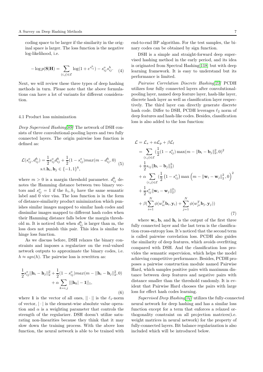4.1 Product loss minimization Deep Supervised Hashing[89] The network of DSH con- sists of three convolutional-pooling layers and two fully connected layers. The origin pairwise loss function is deﬁned as: end-to-end BP algorithm. For the test samples, the bi- nary codes can be obtained by sign function. DSH is a simple and straight-forward deep super- vised hashing method in the early period, and its idea is originated from Spectral Hashing[118] but with deep learning framework. It is easy to understand but its performance is limited. Pairwise Correlation Discrete Hashing[23] PCDH utilizes four fully connected layers after convolutional- pooling layer, named deep feature layer, hash-like layer, discrete hash layer as well as classiﬁcation layer respec- tively. The third layer can directly generate discrete hash code. Diﬀer to DSH, PCDH leverages ℓ2 norm of deep features and hash-like codes. Besides, classiﬁcation loss is also added to the loss function: L = Ls + αLp + βLl L(so ij , dh ij) = 1 2 so ijdh ij + 1 2 (1 − so ij)max(m − dh ij , 0) s.t.hi, hj ∈ {−1, 1}k, (5) + sij kbi − bjk2 2) ( 1 2 (1 − so ij ) max(m − kbi − bjk2 2, 0)2 = X(i,j)∈E where m > 0 is a margin threshold parameter. dh ij de- notes the Hamming distance between two binary vec- tors and so ij = 1 if the hi, hj have the same semantic label and 0 vice visa. The loss function is in the form of distance-similarity product minimization which pun- ishes similar images mapped to similar hash codes and dissimilar images mapped to diﬀerent hash codes when their Hamming distance falls below the margin thresh- old m. It is noticed that when dh ij is larger than m, the loss does not punish this pair. This idea is similar to hinge loss function. As we discuss before, DSH relaxes the binary con- straints and imposes a regularizer on the real-valued network outputs to approximate the binary codes, i.e. h ≈ sgn(h). The pairwise loss is rewritten as: 1 2 ij ||hi − hj||2 so 2 + 1 2 (1 − so ij)max(m − ||hi − hj||2 2, 0) |||hk| − 1||1, + α Xk=i,j (6) where 1 is the vector of all ones, || · || is the ℓ1-norm of vector, | · | is the element-wise absolute value opera- tion and α is a weighting parameter that controls the strength of the regularizer. DSH doesn’t utilize satu- rating non-linearities because they think that it may slow down the training process. With the above loss function, the neural network is able to be trained with 1 2 1 2 1 ( + α X(i,j)∈E 21 − so ij maxm − kwi − wjk2 2 , 02 + ij kwi − wjk2 so 2) N N + β( φ(wT icbi, yi) + φ(wT jcbj, yj)) Xi=1 Xj=1 (7) where wi, bi and hi is the output of the ﬁrst three fully connected layer and the last term is the classiﬁca- tion cross-entropy loss. It’s noticed that the second term is called pairwise correlation loss. PCDH also guides the similarity of deep features, which avoids overﬁtting compared with DSH. And the classiﬁcation loss pro- vides the semantic supervision, which helps the model achieving competitive performance. Besides, PCDH pro- poses a pairwise construction module named Pairwise Hard, which samples positive pairs with maximum dis- tance between deep features and negative pairs with distance smaller than the threshold randomly. It is ev- ident that Pairwise Hard chooses the pairs with large loss for eﬀect hash codes learning. Supervised Deep Hashing[34] utilizes the fully-connected neural network for deep hashing and has a similar loss function except for a term that enforces a relaxed or- thogonality constraint on all projection matrices(i.e. weight matrices in neural network) for the property of fully-connected layers. Bit balance regularization is also included which will be introduced below.

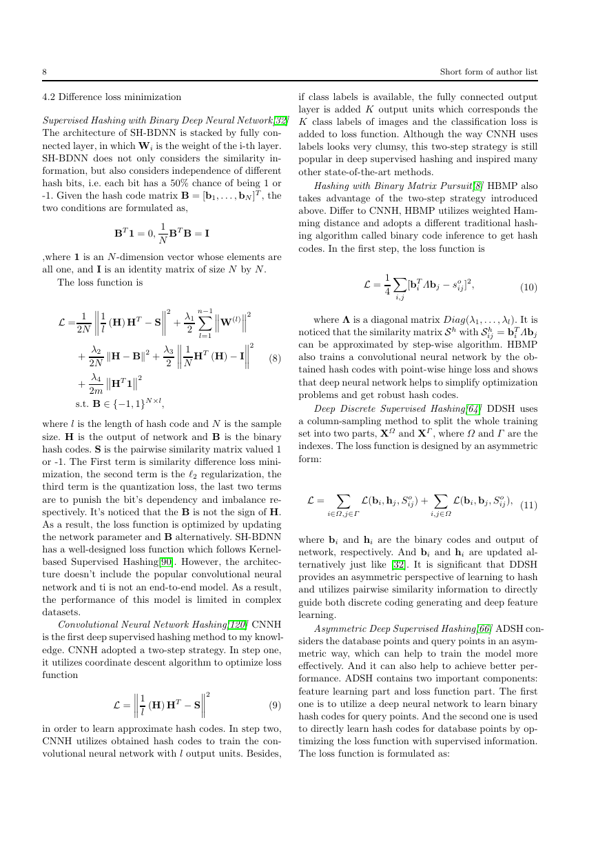
8 4.2 Diﬀerence loss minimization Supervised Hashing with Binary Deep Neural Network[32] The architecture of SH-BDNN is stacked by fully con- nected layer, in which Wi is the weight of the i-th layer. SH-BDNN does not only considers the similarity in- formation, but also considers independence of diﬀerent hash bits, i.e. each bit has a 50% chance of being 1 or -1. Given the hash code matrix B = [b1, . . . , bN ]T , the two conditions are formulated as, BT 1 = 0, 1 N BT B = I ,where 1 is an N -dimension vector whose elements are all one, and I is an identity matrix of size N by N . The loss function is L = 2 + 1 1 l kH − Bk2 + 2N (H) HT − S 2 2mHT 1 s.t. B ∈ {−1, 1}N ×l, λ2 2N λ4 + + λ3 2 λ1 2 1 N n−1 2 2 Xl=1 W(l) HT (H) − I (8) where l is the length of hash code and N is the sample size. H is the output of network and B is the binary hash codes. S is the pairwise similarity matrix valued 1 or -1. The First term is similarity diﬀerence loss mini- mization, the second term is the ℓ2 regularization, the third term is the quantization loss, the last two terms are to punish the bit’s dependency and imbalance re- spectively. It’s noticed that the B is not the sign of H. As a result, the loss function is optimized by updating the network parameter and B alternatively. SH-BDNN has a well-designed loss function which follows Kernel- based Supervised Hashing[90]. However, the architec- ture doesn’t include the popular convolutional neural network and ti is not an end-to-end model. As a result, the performance of this model is limited in complex datasets. Convolutional Neural Network Hashing[120] CNNH is the ﬁrst deep supervised hashing method to my knowl- edge. CNNH adopted a two-step strategy. In step one, it utilizes coordinate descent algorithm to optimize loss function 2 1 l L = (H) HT − S in order to learn approximate hash codes. In step two, CNNH utilizes obtained hash codes to train the con- volutional neural network with l output units. Besides, (9) Short form of author list if class labels is available, the fully connected output layer is added K output units which corresponds the K class labels of images and the classiﬁcation loss is added to loss function. Although the way CNNH uses labels looks very clumsy, this two-step strategy is still popular in deep supervised hashing and inspired many other state-of-the-art methods. Hashing with Binary Matrix Pursuit[8] HBMP also takes advantage of the two-step strategy introduced above. Diﬀer to CNNH, HBMP utilizes weighted Ham- ming distance and adopts a diﬀerent traditional hash- ing algorithm called binary code inference to get hash codes. In the ﬁrst step, the loss function is L = 1 4Xi,j [bT i Λbj − so ij ]2, (10) where Λ is a diagonal matrix Diag(λ1, . . . , λl). It is noticed that the similarity matrix Sh with Sh i Λbj can be approximated by step-wise algorithm. HBMP also trains a convolutional neural network by the ob- tained hash codes with point-wise hinge loss and shows that deep neural network helps to simplify optimization problems and get robust hash codes. ij = bT Deep Discrete Supervised Hashing[64] DDSH uses a column-sampling method to split the whole training set into two parts, XΩ and XΓ , where Ω and Γ are the indexes. The loss function is designed by an asymmetric form: L = Xi∈Ω,j∈Γ L(bi, hj, So ij) + Xi,j∈Ω L(bi, bj, So ij), (11) where bi and hi are the binary codes and output of network, respectively. And bi and hi are updated al- ternatively just like [32]. It is signiﬁcant that DDSH provides an asymmetric perspective of learning to hash and utilizes pairwise similarity information to directly guide both discrete coding generating and deep feature learning. Asymmetric Deep Supervised Hashing[66] ADSH con- siders the database points and query points in an asym- metric way, which can help to train the model more eﬀectively. And it can also help to achieve better per- formance. ADSH contains two important components: feature learning part and loss function part. The ﬁrst one is to utilize a deep neural network to learn binary hash codes for query points. And the second one is used to directly learn hash codes for database points by op- timizing the loss function with supervised information. The loss function is formulated as:

分享到：

赞收藏

资料库

深度哈希方法综述（A Survey on Deep Hashing Methods）.pdf

相关推荐

人工智能

热门标签

最新资料